
Diffusivity#
Diffusivity = {model_name} <species> <float_list> [varies]
Description / Usage#
This required card is used to specify the model for the diffusivity for each species. Definitions of the input parameters are as follows:
{model_name} |
Name of the diffusivity model. This parameter can have one of the following values:
|
<species> |
An integer designating the species equation. |
{float_list} |
the name of the porosity model. One or more floating point numbers (<float1> through <floatn> whose value is determined by the selection for {model_name}. Note that not all the models employ a {float_list}. |
Thus, choices for {model_name} and the accompanying input parameter list are dependent on the {model_name} selected for the Diffusion Constitutive Equation. In some cases, the above model choices have special definitions, while for others some of the above choices do not exist. Thus, the presentation below is keyed to the value chosen for the Diffusion Constitutive Equation model.
When the Diffusion Constitutive Equation model is set to NONE, meaning the material block to which this material file applies is a non-diffusing material, this Diffusivity card should be present in the Material file specification but the model and its parameters will not be used.
For the FICKIAN, GENERALIZED_FICKIAN, DARCY and DARCY_FICKIAN flux models, the following options are valid choices for the Diffusivity {model_name} and accompanying parameter lists.
CONSTANT <species> <float1> |
a constant diffusivity model
|
USER <species> <float_list> |
a user-defined model, the <species> is specified and the set of parameters <float1> through <floatn> is defined by the function usr_diffusivity in the file user_mp.c. |
POROUS <species> <float_list> |
a diffusivity that depends on the saturation and porosity in a porous medium. For two-phase or unsaturated flow in a porous medium, the diffusivity calculated by this model is the diffusivity of solvent vapor through the gas phase in the pore-space This model has been deprecated as the porous equation rewrite has proceeded; it is not recommended for use! |
GENERALIZED <species> <float1> <float2> |
For constant diffusivities used by generalized Fick’s law. The {float_list} consists of two values for each species i or i-j species pair:
|
FREE_VOL <species> <floatlist> |
For a diffusivity determined by free volume theory. The {float_list} for this model contains twelve values:
Note, this model can be run only with a single species equation, i.e., two components |
GENERALIZED_FREE_VOL <species> <floatlist> |
a diffusivity model based on free volume theory and the generalized Fick’s law. This is similar to the FREE_VOL model except it is for a ternary mixture of solvent (1), solvent (2), and polymer (3). A concentration-dependent self-diffusivity is specified. The <species> is defined and the {float_list}, consisting of 12 parameters is identical to and can be specified in the exact same order as in the binary case; see FREE_VOL model above for input parameter list. |
TABLE <integer1> <character_string1> {LINEAR | BILINEAR} [integer2] [FILE = filenm] |
Please see discussion at the beginning of the material properties Chapter 5 for input description and options. Most likely character_string1 will be MASS_FRACTION or TEMPERATURE. |
For the HYDRODYNAMIC flux model (Diffusion Constitutive Equation), there is only one valid choice for the Diffusivity {model_name}, i.e., HYDRO. There are no accompanying parameters but several additional cards are required to define different portions of the model; these cards are identified below. The user is referred to each individual card (identified by italic typeset) definition for the associated model choices and parameter lists.
HYDRO |
For mass transport driven by the hydrodynamic field. No <species> or {float_list} is required, although five additional input cards are required with this diffusivity model. The first specifies Dc in the Shear Rate Diffusivity card. The second specifies Dμ in the Viscosity Diffusivity card. The third specifies Dr in the Curvature Diffusivity card. The fourth specifies the diffusivity of a purely Fickian diffusion mode in the Fickian Diffusivity card; it is usually set to zero. The last card specifies Dg, in the Gravity-based Diffusivity card for the flotation term in variable density transport problems. |
ARRHENIUS <integer 1 <integer 2> <float1> <float2> <float3> |
This is a model for describing effect of temperature on Stefan-Maxwell diffusivities for application in modeling thermal batteries and thus it is used in conjunction with the STEFAN_MAXWELL_CHARGED or STEFAN_MAXWELL flux model (Diffusion Constitutive Equation). Two integers and three floats are required for this diffusivity model:
|
For the FICKIAN_CHARGED flux model (Diffusion Constitutive Equation), only constant diffusivities are allowed. So the Diffusivity model option is:
CONSTANT <species> <float1> |
a constant diffusivity model
|
In addition, the Charge Number and Solution Temperature cards must also be specified in the material file so that the migration flux may be calculated.
The STEFAN_MAXWELL and STEFAN_MAXWELL_CHARGED flux models (Diffusion Constitutive Equation) should be used to model the transport of two or more species only. The diffusivity model for species in these transport problems is currently limited to being CONSTANT and ARRHENIUS. In the CONSTANT& Stefan- Maxwell diffusivity model, a set (only n(n-1)/2 values since Dij = Dji and Dii are not defined) of diffusivities, Dij, is required:
CONSTANT <species> <float1> |
a constant diffusivity model
|
In addition, the Charge Number, Molecular Weight and Solution Temperature cards must also be specified in the material file so that the migration flux may be calculated.
Examples#
Sections of material input files are shown below for several of the Diffusivity model options presented above.
Following is a sample input card for the CONSTANT Diffusivity model:
Diffusivity = CONSTANT 0 1.
Following is a sample section of the material file for the HYDRO Diffusivity model:
Diffusion Constitutive Equation = HYDRODYNAMIC
Diffusivity = HYDRO 0
Shear Rate Diffusivity = LINEAR 0 6.0313e-5
Viscosity Diffusivity = LINEAR 0 6.0313e-5
Curvature Diffusivity = CONSTANT 0 -48.02e-6
Fickian Diffusivity = ANISOTROPIC 0 0. 0.1e-5 0.
Gravity-based Diffusivity = RZBISECTION 0 2.14e-5 5.1 0.5 0.5
Following is a sample section of the material file for the GENERALIZED_FREE_VOL Diffusivity model:
Diffusion Constitutive Equation = GENERALIZED_FICKIAN
Diffusivity = GENERALIZED_FREE_VOL 1 0.943 1.004 0.000983 0.000239 -12.12 -96.4 0.395 0.266 0.00143 0 1.265983036 0.9233610342
Sample section of the material file for the STEFAN_MAXWELL_CHARGED Diffusion Constitutive Equation with the CONSTANT Diffusivity model:
Diffusion Constitutive Equation = STEFAN_MAXWELL_CHARGED
Diffusivity = CONSTANT
0 1 2.0e-05
0 2 2.0e-05
1 2 2.0e-05
Solution Temperature = THERMAL_BATTERY 846. 298. .03 7.7 0.6 1030.
Molecular Weight = CONSTANT 0 6.939
Charge Number = CONSTANT 0 1.0
Molecular Weight = CONSTANT 1 39.098
Charge Number = CONSTANT 1 1.0
Molecular Weight = CONSTANT 2 35.4
Charge Number = CONSTANT 2 -1.0
Sample section of the material file for the STEFAN_MAXWELL_CHARGED Diffusion Constitutive Equation with the ARRHENIUS Diffusivity model:
0 1 1.5e-05 80000.0 846.0
0 2 1.5e-05 80000.0 846.0
1 2 1.5e-05 80000.0 846.0
(the Charge Number, Molecular Weight and Solution Temperature cards are similarly specified as above in the CONSANT Diffusivity case)
Technical Discussion#
Following are brief comments on the various Diffusivity models.
POROUS For this model, diffusivity depends on the saturation and porosity in a porous medium. For two-phase or unsaturated flow in a porous medium, the diffusivity calculated by this model is the diffusivity of solvent vapor through the gas phase in the pore-space (see Martinez, 1995). However as indicated above, this model is not recommended for use at his time.
GENERALIZED This model generalizes Fick’s Law for multicomponent diffusion. The elements along the diagonal, Dii, are self-diffusivities, while Dij are mutual diffusivities between species i and j. Note that mutual diffusivities in generalized formulation can be both positive and negative, and are constant values.
FREE_VOL For a diffusivity determined by free volume theory (cf. Duda et al. 1982). In mathematical form, the binary mutual diffusion coefficient (solvent diffusion in a polymeric solution), using the free volume theory, is given by:
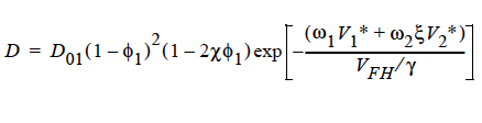
where
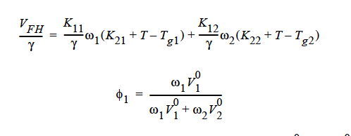
Here, ω1 is the solvent weight fraction, ω2 polymer weight fraction; V0 1 and V02 are, respectively, solvent and polymer specific volumes; φ1 solvent volume fraction, φ2 polymer volume fraction; γ overlap factor to account for shared free volume; Tg1 and Tg2 respectively solvent and polymer glass transition temperature, T absolute temperature; K11, K12, K21 and K22 solvent free-volume parameters; V* 1 and V*2 respectively, solvent and polymer specific critical-hole volumes; D01 constant preexponential factor when E is presumed to be zero (E is energy required to overcome attractive forces from neighboring molecules); ξ ratio of solvent and polymer jumping units; and χ Flory-Huggins polymer/solvent interaction parameter. In general, D01 should be expressed as D01 e- E/RT with R being the universal gas constant. Dependence of diffusivity, D, on temperature and mass fraction can be determined once the above twelve parameters are specified.
Note: This model (FREE_VOL) can be run ONLY with 1 species equation, i.e., with two components.
GENERALIZED_FREE_VOL This is a diffusivity model based on free volume theory and the generalized Fick’s law. For a ternary mixture of solvent (1), solvent (2), and polymer (3), the concentration-dependent self-diffusivity is given by (Vrentas, et. al., 1984):
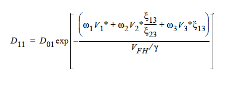
where
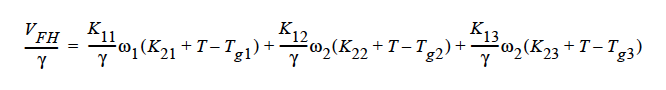
The parameters for this model are the same twelve parameters as for the binary FREE_VOL model and so can be specified in the exact same order. The mutual diffusivities required to fill the cross-terms are also concentration-dependent. In addition, the gradient in chemical potential is also accounted for (Alsoy and Duda, 1999; Zielinski and Hanley, 1999).
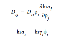
ai is the activity of species i, which can be written in terms of the activity coefficient, γi, and volume fraction, φi. The current implementation of species activity is based on the Flory-Huggins model for multicomponent polymer-solvent mixtures (Flory, 1953).
HYDRO implies that mass transport of at least one species is driven by gradients in the second invariant of the rate of deformation tensor (shear rate) and gradients in viscosity (Phillips, et.al. 1992). This model also includes a sedimentation flux term to account for the motion of non-neutrally buoyant particles resulting from gravitation (Zhang and Acrivos, 1994) and a curvature-driven flux term from normal component of the acceleration vector (Krishnan, et. al., 1996). This model is used in predicting the particle distributions of particulate suspensions undergoing flow. For this model, the mass flux vector J is given by the following:
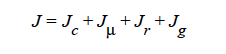
where
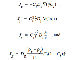
where Ci is the particulate phase volume fraction, i is the species number designation of the particulate phase, the shear rate, μ the viscosity, the normal unit acceleration vector, r the curvature of streamlines, Dc, Dμ, Dr and Dg the “diffusivity” parameters, ρs and ρf the particle and fluid phase densities, respectively, and , the gravitational acceleration vector.
ARRHENIUS Diffusivities can be strongly dependent on temperature as in processes such as thermal batteries. Such temperature dependency can be described using the following constitutive model that makes use of Arrhenius temperature dependency:
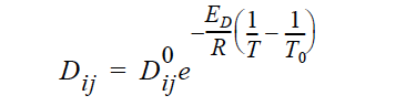
where Dij are the Stefan-Maxwell diffusivities as defined in Equations 13 and 14. are the reference Stefan-Maxwell diffusivities at reference temperature T0; ED is the activation energy that controls the temperature dependency and R is the universal gas constant; and T is temperature. The units of ED, R and T are such that is dimensionless.
STEFAN-MAXWELL For multicomponent diffusion of neutral species in concentrated solutions. The Stefan-Maxwell diffusivities, Dij, as defined in the following Stefan-Maxwell flux model (cf. Chen, et. al., 2000, Chen, et. al., 1998):
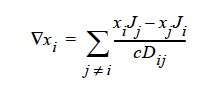
are taken to be constant. Here, xi is mole fraction of species i, Ji the molar flux of species i, and c the total molar concentration. Since Dij = Dji and Dii are not defined, only n(n-1)/2 Stefan-Maxwell diffusivities are required (here, n is the total number of diffusing species). For example, for n = 3 (i.e., a solution having three species), three Stefan-Maxwell diffusivities are needed: D12, D13, and D23.
STEFAN-MAXWELL_CHARGED For multicomponent transport (diffusion and migration) of charged species in concentrated electrolyte solutions. The Stefan- Maxwell diffusivities, Dij, as defined in the following Stefan-Maxwell flux model (cf. Chen et al. 2002, Chen, et. al., 2000, Chen, et. al., 1998):
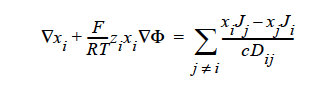
are taken to be constant, as in the case of multicomponent diffusion of neutral species in concentrated solutions. Here, Φ is electrical potential in electrolyte solution, zi charge number of species i, F Faraday constant (96487 C/mole), R universal gas constant (8.314 J/mole-K), and T electrolyte solution temperature.
FICKIAN_CHARGED For multicomponent transport (diffusion and migration) of charged species in dilute electrolyte solutions. The Fickian diffusivity of species i, Di, as defined in the following Fickian flux model (cf. Newman, 1991; Chen, et. al., 2000):
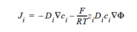
is taken to be constant. Here, ci is molar concentration of species i.
FAQs#
The following is a discussion of Units in Goma but covers several important Diffusionrelated items. It comes from some emails exchanged at Sandia during January 1998; while the discussions are relevant for each user of the code, the deficiencies or lack ofclarity have been since been remedied prior to Goma 4.0.
Unit Consistency in Goma (Jan 98)
Question:… I know what you are calling volume flux is mass flux divided by density. The point I am trying to make is that the conservation equations in the books I am familiar with talk about mass, energy, momentum, and heat fluxes. Why do you not write your conservation equations in their naturally occurring form? If density just so happens to be common in all of the terms, then it will be obvious to the user that the problem does not depend on density. You get the same answer no matter whether you input rho=1.0 or rho=6.9834, provided of course this does not impact iterative convergence. This way, you write fluxes in terms of gradients with the transport properties (viscosity, thermal conductivity, diffusion coefficient, etc.) being in familiar units.
Answer: First let me state the only error in the manual that exists with regard to the convection-diffusion equation (CDE) is the following:
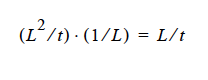
Ji in the nomenclature table should be described as a volume flux with units of L/t, i.e. D ⋅ ∇yi, where D is in L2/t units.
Now, this is actually stated correctly elsewhere, as it states the Ji is a diffusion flux (without being specific); to be more specific here, we should say it is a “volume flux of species i.” So, in this case D is in L ⋅ L ⁄ t units, yi is dimensionless and it is immaterial that the CDE is multiplied by density or not, as long as density is constant.
Now, in Goma we actually code it with no densities anywhere for the FICKIAN diffusion model. For the HYDRO diffusion model, we actually compute a Ji ⁄ ρ in the code, and handle variable density changes through that . In that case Ji as computed in Goma is a mass flux vector, not a volume flux vector, but by dividing it by and sending it back up to the CDE it changes back into a volume flux. i. e., everything is the same.
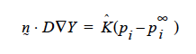
Concerning the units of the mass transfer coefficient on the YFLUX boundary condition, the above discussion now sets those. Goma clearly needs the flux in the following form:
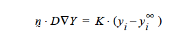
and dimensionally for the left hand side
where D is in units L2 ⁄ t, the gradient operator has units of 1 ⁄ L so K has to be in units of L ⁄ t (period!) because yi is a fraction.
then K’s units will have to accommodate for the relationship between p1 and y1 in the liquid, hopefully a linear one as in Raoult’s law, i.e. if pi = PVyi where pv is the vapor pressure, then
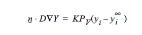
and so K on the YFLUX command has to be KPv ….and so on.
Finally, you will note, since we do not multiply through by density, you will have to take care of that, i. e., in the Price paper (viz., Price, et. al., 1997) he gives K in units of t ⁄ L. So, that must be converted as follows:
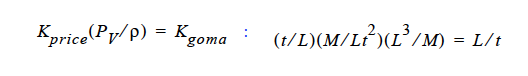
This checks out!
References#
Alsoy, S. and Duda, J. L., 1999. “Modeling of Multicomponent Drying of Polymer Films.” AIChE Journal, (45)4, 896-905.
Chen, K. S., Evans, G. H., Larson, R. S., Noble, D. R. and Houf, W. G. “Final Report on LDRD Project: A Phenomenological Model for Multicomponent Transport with Simultaneous Electrochemical Reactions in Concentrated Solutions”, SAND2000- 0207, Sandia National Laboratories Technical Report (2000).
Chen, K. S., Evans, G. H., Larson, R. S., Coltrin, M. E. and Newman, J. “Multidimensional modeling of thermal batteries using the Stefan-Maxwell formulation and the finite-element method”, in Electrochemical Society Proceedings, Volume 98-15, p. 138-149 (1998).
Chen, K. S., “Modeling diffusion and migration transport of charged species in dilute electrolyte solutions: GOMA implementation and sample computed predictions from a case study of electroplating”, Sandia memorandum, September 21, 2000.
Chen, K. S., Evans, G. H., and Larson, R. S., “First-principle-based finite-element modeling of a Li(Si)/LiCl-KCl/FeS2 thermal battery cell”, in Electrochem. Soc. Proc. Vol. 2002-30, p. 100 (2002).
Duda, J. L., Vrentas, J. S., Ju, S. T. and Liu, H. T. 1982. “Prediction of Diffusion Coefficients for Polymer-Solvent Systems”, AIChE Journal, 28(2), 279-284.
P.J. Flory, Principles of Polymer Chemistry, Cornell University Press, 1953. Krishnan, G. P., S. Beimfohr and D. Leighton, 1996. “Shear-induced radial segregation in bidisperse suspensions,” J. Fluid Mech. 321, 371.
Martinez, M. M., Mathematical and Numerical Formulation of Nonisothermal Multicomponent Three-Phase Flow in Porous Media, SAND95-1247, Sandia National Laboratories Technical Report, 1995.
Newman, J. S., Electrochemical Systems, Prentice Hall, Inc., Englewood Cliffs, New Jersey (1991).
Phillips, R.J., R.C. Armstrong and R.A. Brown, 1992, “A constitutive equation for concentrated suspensions that accounts for shear-induced particle migration,” Physics of Fluids A, 4(1), 30-40.
Price, P. E., Jr., S. Wang, I. H. Romdhane, “Extracting Effective Diffusion Parameters from Drying Experiments,” AIChE Journal, 43, 8, 1925-1934 (1997)
Vrentas, J.S., J.L. Duda and H.-C. Ling, 1984. “Self-Diffusion in Polymer-Solvent- Solvent Systems” Journal of Polymer Sciences: Polymer Physics edition, (22), 459- 469.
Zhang K. and A. Acrivos, 1994, “Viscous resuspension in fully-developed laminar pipe flows,” Int. J. Multiphase Flow, (20)3, 579-591.
Zielinski, J.M. and B.F. Hanley, 1999. “Practical Friction-Based Approach to Modeling Multicomponent Diffusion.” AIChE Journal, (45)1, 1-12.