Liquid Constitutive Equation

Liquid Constitutive Equation = {model_name}

Description / Usage

This required card is used to specify the stress, strain-rate/strain constitutive equation associated with the momentum equations (e.g. Navier-Stokes equations) and contains Newtonian and generalized Newtonian models. The single input parameter is the {model_name} with the options listed below:

{model_name}

Name of the constitutive equation, being one of the following values: NEWTONIAN, POWER_LAW, CARREAU, BINGHAM, CARREAU_WLF, CURE, THERMAL, EPOXY, SUSPENSION, FILLED_EPOXY, POWERLAW_SUSPENSION, CARREAU_SUSPENSION, or HERSCHEL_BULKLEY. Each of these constitutive models require additional parameters that are entered via additional cards, as described below.

Thus,

NEWTONIAN

For a simple constant viscosity Newtonian fluid. This model requires one floating point value,

\(\mu\), where \(\mu\) is the viscosity in the chosen units for the problem and is entered with the Viscosity card.

POWER_LAW

For a power law model. This model requires two parameters. The first, μ0, is the zero strain-rate limit of the viscosity and is entered with the Low Rate Viscosity card. The second, n, is the exponent on the strain rate which can take on any value between 1 (Newtonian) and 0 (infinitely shear thinning). n is entered with the Power Law Exponent card. The form of the equation is

where is the second invariant of the shear-rate tensor. To obtain solutions with the power law model, it is best to start with a Newtonian initial guess since the viscosity becomes infinite at zero shear-rate.

CARREAU

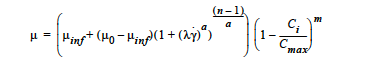
For a Carreau-Yasuda strain-rate thinning or thickening relation. This option requires five floating point values. The first, μ0, is the zero strain-rate limit of the viscosity and is entered with the Low Rate Viscosity card. The second, n, is the exponent on the strain rate which can take on any value between 1 (Newtonian) and 0 (infinitely shear thinning). n is entered with the Power Law Exponent card. The third, μinf, is the high-strainrate limit to the viscosity and is entered with the High Rate Viscosity card. The fourth, λ, is the time constant reflecting the strain-rate at which the transition between μ0 and μinf takes place. λ is entered with the Time Constant card. The fifth, a, is a dimensionless parameter that describes the transition between the low-rate and the power-law region and is entered with the Aexp card. The form of the equation is

where is the second invariant of the shear-rate tensor.

BINGHAM

For a Bingham-Carreau-Yasuda fluid. This option requires eight floating point values. It uses the same parameters as the CARREAU model with the addition of coefficients to describe the yield and temperature dependent behavior. The first, μ0, is the zero strain-rate limit of the viscosity and is entered with the Low Rate Viscosity card. The second, n, is the exponent on the strain rate which can take on any value between 1 (Newtonian) and 0 (infinitely shear thinning). n is entered with the Power Law Exponent card. The third, μinf, is the high-strain-rate limit to the viscosity and is entered with the High Rate Viscosity card. The fourth, λ, is the time constant reflecting the strain-rate at which the transition between μ0 and μinf takes place. λ is entered with the Time Constant card. The fifth, a, is a dimensionless parameter that describes the transition between the low-rate and the power-law region and is entered with the Aexp card. The form of the equation is

where is a simplified temperature dependent shift factor that is expressed as an Arrhenius type temperature dependence of the following form:

The exponent for the temperature dependence, Eμ/R, is input using the Thermal Exponent card. Tref is input using the Reference Temperature card in the thermal properties section of the material file. The stress at which the material yields is input with the Yield Stress card. The sharpness of the transition from the solid to fluid state, F, is indicated with the Yield Exponent card.

CARREAU_WLF

An extension of the Carreau-Yasuda model to incorporate a temperature-dependent shift in shear-rate according to the Williams-Landel-Ferry equation (Hudson and Jones, 1993). The form of the equation is

where \(a_T\) is another form of the temperature-dependent shift factor:

Here is a thermal exponential factor (can be Arrhenius) and is input by the Thermal Exponent card; \(c_2\) is the WLF constant 2 and is input by the Thermal WLF Constant2 card. μ0, is the zero strain-rate limit of the viscosity and is entered with the Low Rate Viscosity card. n, is the exponent on the strain rate which can take on any value between 1 (Newtonian) and 0 (infinitely shear thinning) and is entered with the Power Law Exponent card. \(μ_{inf}\), is the high-strain-rate limit to the viscosity and is entered with the High Rate Viscosity card. λ, is the time constant reflecting the strain-rate at which the transition between μ0 and μinf takes place and is entered with the Time Constant card. a, is a dimensionless parameter that describes the transition between the low-rate and the power-law region and is entered with the Aexp card.

CURE

For a model to increase the viscosity with the extent of reaction. The Cure model can be used to represent polymerizing systems whose viscosity depends on the extent of reaction. The form of the equation is

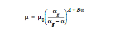
This option requires four floating point values. The first, μ0, is the reference state viscosity and is entered with the Low Rate Viscosity card. The constant, \(α_g\), is entered with the Cure Gel Point card and marks the extent of reaction at the transition from the liquid to the solid state. The exponents A and B are entered with the Cure A Exponent and Cure B Exponent cards.

THERMAL

For a temperature-dependent viscosity. This option, which requires two floating point values, can be used to represent fluids that change viscosity with temperature. The form of the equation is

where the reference state viscosity, μ0, is entered with the Low Rate Viscosity card. The exponent, Eμ/R, is specified using the Thermal Exponent card.

EPOXY

For a thermal and curing component. The Epoxy model combines the temperature dependence of the THERMAL option with the extent of reaction dependence of the CURE option. The functional form of the equation is:

Five cards must be used to specify all the parameters for this model. The first, μ0, is the reference state viscosity and is entered with the Low Rate Viscosity card. The thermal exponent, Eμ/R, is specified using the Thermal Exponent card. The constant, \(α_g\), is entered with the Cure Gel Point card and marks the extent of reaction at the transition from the liquid to the solid state. The exponents A and B are entered with the Cure A Exponent and Cure B Exponent cards.

SUSPENSION

For simulating a carrier fluid with high-volume fraction particles. This option invokes a concentrationdependent viscosity model useful in modeling solid suspensions. The functional form associated with this option is,

where μ0 is effectively the viscosity of the suspending fluid specified with the Low Rate Viscosity card, n is an exponent specified by the Power Law Exponent card and is typically less than zero. \(C_{max}\) is the “binding” solid concentration and is specified with the Suspension Maximum Packing card. Ci is the solid concentration and is tied to a convective-diffusion equation specified in the equation section of the Problem Description. The correct species number “i” is specified with the Suspension Species Number card. Note that for \(C_i\) > \(C_{max}\) and n < 0, the model as written above is physically undefined. For concentrations in this range, a very large value for viscosity will be used, effectively solidifying the material.

FILLED_EPOXY

This option combines the cure and thermal dependence of the EPOXY model with the solid volume fraction dependence of the SUSPENSION model. The functional form of this equation is

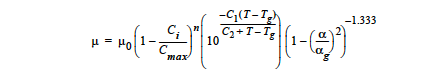
with the temperature \(T_g\) being calculated from

Here the viscosity now depends on extent of reaction, temperature and solid volume fraction. Nine cards must be specified to define the parameters for this option and are entered in the following manner. The first, μ0, is the reference state viscosity and is entered with the Low Rate Viscosity card. n is the exponent for suspension behavior and is specified by the Power Law Exponent card; it is typically less than zero. \(C_{max}\) is the “binding” solid concentration and is specified with the Suspension Maximum Packing card. \(C_i\) is the solid concentration and is tied to a convective-diffusion equation specified in the equation section of the previous chapter. The correct species number “i” is identified with the Suspension Species Number card. Here \(c_1\) is a thermal exponential factor and is input by the Thermal Exponent card; \(c_2\) is a second thermal exponent and is entered via the Cure B Exponent card. The constant for the curing model, \(α_g\), is entered with the Cure Gel Point card and marks the extent of reaction at the transition from the liquid to the solid state. The cure exponent used in the EPOXY model is here assumed to be constant (-4/3) and is fixed in the model. The constant A in the gel temperature equation is entered with the Cure A Exponent card and the temperature is entered with the Unreacted Gel Temperature card. Although it does not appear directly in the model equations, the Cure Species Number must also be specified.

POWERLAW_SUSPENSION

This is a specialized research model that incorporates the power law model with the suspension model to try and simulate particles suspending in shear-thinning fluid. This option requires five input values. The first, μ0, is the zero strain-rate limit of the viscosity of the solvent and is entered with the Low Rate Viscosity card. The second, n, is the exponent on the strain rate which can take on any value between 1 (Newtonian) and 0 (infinitely shear thinning). n is entered with the Power Law Exponent card. The third value is the exponent for the suspension Krieger model, which is input through the Thermal Exponent, m. The fourth term is the suspension maximum packing, \(C_{max}\), which is entered through the Suspension Maximum Packing card. \(C_i\) is the solid concentration and is tied to a convectivediffusion equation specified in the equation section of the previous chapter. The correct species number “i” is identified with the Suspension Species Number card. The form of the equation is

where y is the second invariant of the shear-rate tensor. It is best to start with a Newtonian initial guess for the power law suspension model, since the viscosity for the power law model will become infinite at zero shear-rate.

CARREAU_SUSPENSION

This model is a hybrid for the flow of particle-laden suspensions in shear-thinning fluids. It uses a Carreau-Yasuda strain-rate thinning or thickening relation for the suspending fluid and a Krieger model for the suspension. This option requires eight input values. The first, μ0, is the zero strain- rate limit of the viscosity and is entered with the Low Rate Viscosity card. The second, n, is the exponent on the strain rate which can take on any value between 1 (Newtonian) and 0 (infinitely shear thinning). n is entered with the Power Law Exponent card. The third, μinf, is the high-strain-rate limit to the viscosity and is entered with the High Rate Viscosity card. The fourth, λ, is the time constant reflecting the strain-rate at which the transition between μ0 and μinf takes place. λ is entered with the Time Constant card. The fifth, a, is a dimensionless parameter that describes the transition between the low-rate and the power-law region and is entered with the Aexp card. The sixth value is the exponent for the suspension Krieger model, which is input through the Thermal Exponent, m. The seventh term is the suspension maximum packing, Cmax, which is entered through the Suspension Maximum Packing card. Ci is the solid concentration and is tied to a convective-diffusion equation specified in the equation section of the previous chapter. The correct species number “i” is identified with the Suspension Species Number card.The form of the equation is

where y is the second invariant of the shear-rate tensor.

HERSCHEL_BULKLEY

This is a variant on the power law model that includes a yield stress. It requires three input values to operate: a reference viscosity value, μ0, a power-law exponent, n. and a yield shear stress value, \(τ_y\). The model for this constitutive relations is as follows:

The nature of this relation is best seen by multiplying the entire relation by the shear rate to produce a relation between shear stress and shear rate. In this manner it can be seen that the shear stress does not go to zero for zero shear rate. Instead it approaches the yield shear stress value. Put another way, only for imposed shear stresses greater than the yield stress will the fluid exhibit a nonzero shear rate. This is effective yielding behavior.

A caveat needs stating at this point. This model is essentially a superposition of two power-law models. One with the supplied exponent and the other with an implicit exponent of n = 0. It has long been observed that power-law models with exponents approaching zero exhibit very poor convergence properties. The Herschel_Bulkley model is no exception. To alleviate these convergence problems somewhat, the sensitivities of the yield stress term with respect to shear rate has not been included in the Jacobian entries for this viscosity model. This helps in that it allows for convergence at most yield stress values, but also means that the iteration scheme no longer uses an exact Jacobian. The difference is seen in that this model will take relatively more iterations to converge to an answer. The user should expect this and not be too troubled (it’s alright to be troubled a little).

TURBULENT_SA

Spalart Allmaras turbulence model. This model is a one-equation model. The viscosity term is the kinematic viscosity, thus density should be 1.

Wall functions are expected to be provided in an external field DIST or see turbulence documentation on how to calculate wall distance in goma.

TURBULENT_SA_DYNAMIC

Same as TURBULENT_SA but multiplies kinematic viscosity by density in the momentum equation to get a dynamic viscosity.

Examples

The following is a sample card setting the liquid constitutive equation type to NEWTONIAN and demonstrates the required cards:

Liquid Constitutive Equation = NEWTONIAN

Viscosity = CONSTANT 1.00

The following is a sample card setting the liquid constitutive equation type to POWER_LAW and demonstrates the required cards:

Liquid Constitutive Equation = POWER_LAW

Low Rate Viscosity= CONSTANT 1.

Power Law Exponent= CONSTANT 1.

The following is a sample card setting the liquid constitutive equation type to CARREAU and demonstrates the required cards:

Liquid Constitutive Equation = CARREAU

Low Rate Viscosity= CONSTANT 1.

Power Law Exponent= CONSTANT 1.

High Rate Viscosity= CONSTANT 0.001

Time Constant = CONSTANT 1.

Aexp = CONSTANT 1.

The following is a sample card setting the liquid constitutive equation type to BINGHAM and demonstrates the required cards:

Liquid Constitutive Equation = BINGHAM

Low Rate Viscosity= CONSTANT 10.00

Power Law Exponent= CONSTANT .70

High Rate Viscosity= CONSTANT 0.01

Time Constant = CONSTANT 100.

Aexp = CONSTANT 2.5

Thermal Exponent = CONSTANT 1.

Yield Stress = CONSTANT 5.

Yield Exponent = CONSTANT 1.0

Reference Temperature= CONSTANT 273.

The following is a sample card setting the liquid constitutive equation type to CARREAU_WLF and demonstrates the required cards:

Liquid Constitutive Equation = CARREAU_WLF

Low Rate Viscosity= CONSTANT 10.00

Power Law Exponent= CONSTANT .70

High Rate Viscosity= CONSTANT 0.01

Time Constant = CONSTANT 100.

Aexp = CONSTANT 2.5

Thermal Exponent = CONSTANT 1.

Thermal WLF Constant2 = CONSTANT 0.5

Reference Temperature= CONSTANT 273.

The following is a sample card setting the liquid constitutive equation type to CURE and demonstrates the required cards:

Liquid Constitutive Equation = CURE

Low Rate Viscosity= CONSTANT 1.

Power Law Exponent= CONSTANT 1.

The following is a sample card setting the liquid constitutive equation type to THERMAL and demonstrates the required cards:

Liquid Constitutive Equation = THERMAL

Low Rate Viscosity= CONSTANT 1.

Thermal Exponent= CONSTANT 9.

The following is a sample card setting the liquid constitutive equation type to EPOXY and demonstrates the required cards:

Liquid Constitutive Equation = EPOXY

Liquid Constitutive Equation = FILLED_EPOXY

Low Rate Viscosity= CONSTANT 1.e5

Thermal Exponent= CONSTANT 9.

Cure Gel Point = CONSTANT 0.8

Cure A Exponent= CONSTANT 0.3

Cure B Exponent= CONSTANT 43.8

The following is a sample card setting the liquid constitutive equation type to SUSPENSION and demonstrates the required cards:

Liquid Constitutive Equation = SUSPENSION

Low Rate Viscosity= CONSTANT 1.e5

Power Law Exponent = CONSTANT -3.0

Suspension Maximum Packing= CONSTANT 0.49

Suspension Species Number = 0

The following is a sample card setting the liquid constitutive equation type to FILLED_EPOXY and demonstrates the required cards:

Liquid Constitutive Equation = FILLED_EPOXY

Low Rate Viscosity = CONSTANT 1.e5

Power Law Exponent = CONSTANT -3.0

Thermal Exponent = CONSTANT 9.

Suspension Maximum Packing = CONSTANT 0.49

Suspension Species Number = 0

Cure Gel Point = CONSTANT 0.8

Cure A Exponent = CONSTANT 0.3

Cure B Exponent = CONSTANT 43.8

Cure Species Number = 2

Unreacted Gel Temperature = CONSTANT 243

The following is a sample card setting the liquid constitutive equation type to POWERLAW_SUSPENSION and demonstrates the required cards:

Liquid Constitutive Equation = POWERLAW_SUSPENSION

Low Rate Viscosity= CONSTANT 1.

Power Law Exponent= CONSTANT 1.

Thermal Exponent = CONSTANT -1.82

Suspension Maximum Packing= CONSTANT 0.68

Suspension Species Number= 0

The following is a sample card setting the liquid constitutive equation type to CARREAU_SUSPENSION and demonstrates the required cards:

Liquid Constitutive Equation = CARREAU_SUSPENSION

Low Rate Viscosity= CONSTANT 1.

Power Law Exponent= CONSTANT 1.

High Rate Viscosity= CONSTANT 0.001

High Rate Viscosity= CONSTANT 0.001

Time Constant = CONSTANT 1.

Aexp = CONSTANT 1.

Thermal Exponent = CONSTANT -1.82

Suspension Maximum Packing= CONSTANT 0.68

Suspension Species Number= 0

The following card gives an example of the HERSCHEL_BULKLEY model

Liquid Constitutive Equation = HERSCHEL_BULKLEY

Low Rate Viscosity = CONSTANT 0.337

Power Law Exponent = CONSTANT 0.817

Yield Stress = CONSTANT 1.39

Technical Discussion

See Description/Usage section for this card.

Theory

The NEWTONIAN, POWER_LAW, and CARREAU models are described in detail in Bird, et al. (1987). Details of the continuous yield stress model used in the Bingham- Carreau-Yasuda (BINGHAM) model, which is a Carreau model combined with a continuous yield stress model, can be found in Papanastasiou (1987).

References

Bird, R. B., Armstrong, R. C., and Hassager, O. 1987. Dynamics of Polymeric Liquids, 2nd ed., Wiley, New York, Vol. 1.

Hudson, N. E. and Jones, T. E. R., 1993. “The A1 project - an overview”, Journal of Non-Newtonian Fluid Mechanics, 46, 69-88.

Papanastasiou, T. C., 1987. “Flows of Materials with Yield,” Journal of Rheology, 31 (5), 385-404.

Papananstasiou, T. C., and Boudouvis, A. G., 1997. “Flows of Viscoplastic Materials: Models and Computation,” Computers & Structures, Vol 64, No 1-4, pp 677-694.