PARTICLE#

PARTICLE = <float_list> <file_name>

Description / Usage#

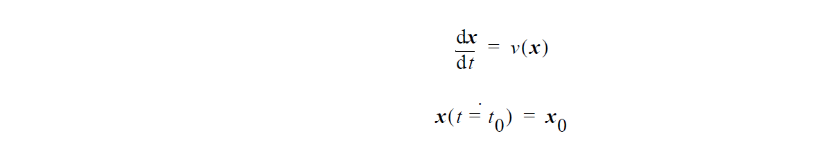
Each PARTICLE card represents a separate particle trajectory. As many of these cards as desired can be input to direct Goma to compute a particle trajectory.

There are eleven values to specify in the <float_list>; definitions of the input parameters are as follows:

<float1>	xpt, the X-coordinate of the origin of the trajectory.
<float2>	ypt, the Y-coordinate of the origin of the trajectory.
<float3>	zpt, the Z-coordinate of the origin of the trajectory.
<float4>	initial_time, the start time for computing the trajectory (a value in units consistent with rest of the problem, i.e. length scale/velocity scale).
<float5>	end_time, the end time for computing the trajectory. The trajectory will be computed until the end time is reached or until the particle trajectory leaves the computational domain.
<float6>	point_spacing, the desired distance between successive points on the trajectory. The point spacing may be decreased below this value if required by the trajectory calculation but it will not exceed it.
<float7>	mobility, the mobility of the particle when particles with inertia are desired. Enter zero for inertia-less trajectories.
<float8>	mass, the mass of the particle. If the trajectory of an inertialess particle is desired, a value of 0.0 should be entered.
<float9>	force_x, the X-component of an external force (such as gravity) which is to be applied to the particle (with mass).
<float10>	force_y, the Y-component of an external force (such as gravity) which is to be applied to the particle (with mass).
<float11>	force_z, the Z-component of an external force (such as gravity) which is to be applied to the particle (with mass).
<file_name>	A character string corresponding to a file name into which the output should be printed.

Thus, the particle trajectory starts at the coordinates defined by xpt, ypt, and zpt. The trajectory of the particle is computed starting at a time value of initial_time and continuing until end_time is reached or until the particle exits the computational domain. The time step is adjusted so that the distance between successive points on the trajectory is, at most, equal to the point_spacing (it may be less if the time-stepping algorithm requires it). At each point along the trajectory, the usr_ptracking routine is called which the user may modify to control the output to file_name.

Examples#

Here is an example of an input deck with 6 trajectory cards.

Post Processing Particle Traces =
PARTICLE = -1.8 -0.1 3.0 0 10000 0.02 0 0 0 0 0 part1.out
PARTICLE = -1.8 -0.1 3.0 0 1000 0.02 {mob1} {mass1} 0 {-f1} 0 part1.out
PARTICLE = -1.8 -0.1 3.0 0 1000 0.02 {mob2} {mass2} 0 {-f2} 0 part1.out
PARTICLE = -1.8 -0.15 3.0 0 10000 0.02 0 0 0 0 0 part2.out
PARTICLE = -1.8 -0.15 3.0 0 1000 0.02 {mob1} {mass1} 0 {-f1} 0 part2.out
PARTICLE = -1.8 -0.15 3.0 0 1000 0.02 {mob2} {mass2} 0 {-f2} 0 part2.out
END OF PARTICLES

Technical Discussion#

The vorticity vector function, \(\underline\omega\) , is defined in terms of the velocity \(\underline\upsilon\) as:

Trapezoidal rule time integration is utilized with Euler prediction.

For trajectories with particle inertia (i.e. when the product of mass and mobility is greater than zero), the following evolution equation is used:

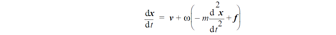
where \(\omega\) is the particle mobility (e.g. 1 ⁄ (\(6\pi\mu r\)) for a sphere of radius r in a liquid of viscosity \(\mu\) ), m is the particle mass, and f is the external force vector acting on the particle.

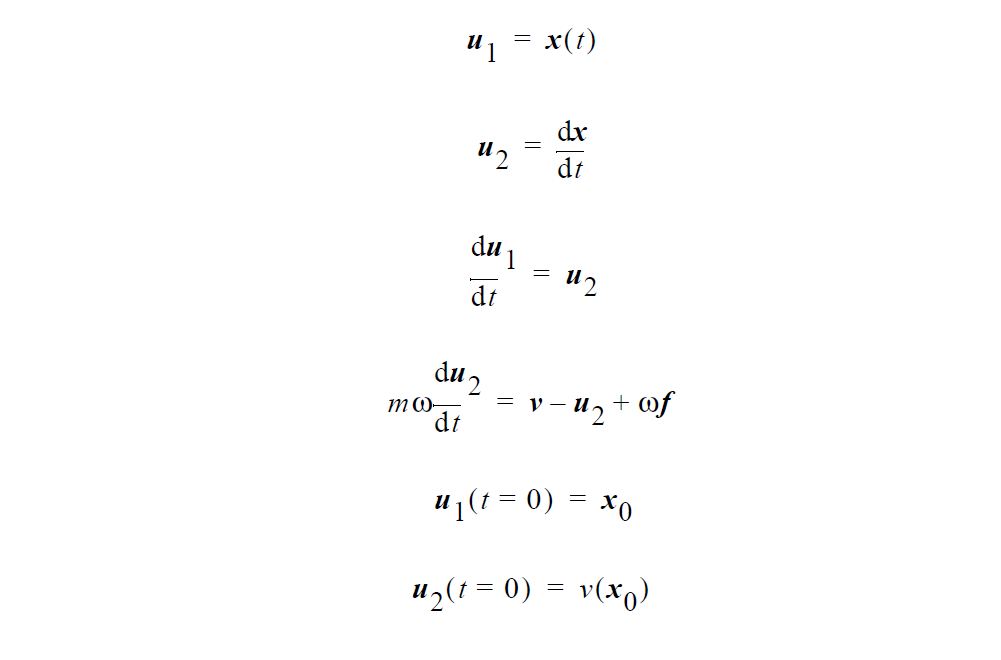
The trajectory is computed using a coupled set of ordinary differential equations:

References#

Russel, Saville, and Schowalter, Colloidal Dispersions, pp. 374-377.