
Category 6: Mass Equations#
The collection of boundary conditions in this category are applied to the mass balance equations, specifically the species component balance equations. Most boundary conditions are weakly integrated conditions defining fluxes at internal or external surfaces, although strongly integrated and Dirichlet conditions are also available to control known values of dependent variables or integrated quantities. Boundary conditions are available for chemical species as well as charged species, suspensions and liquid metals. An important capability in Goma is represented by the discontinuous variable boundary conditions, for which users are referred to Schunk and Rao (1994) and Moffat (2001). Care must be taken if the species concentration is high enough to be outside of the dilute species assumption, in which case transport of species through boundaries will affect the volume of the bounding fluids. In these cases, users are referred to the VNORM_LEAK condition for the fluid momentum equations and to KIN_LEAK for the solid momentum (mesh) equations. And finally, users are cautioned about different bases for concentration (volume, mass, molar) and several discussions on or references to units.
Y#
BC = Y NS <bc_id> <integer> <float1> [float2] [integer2]
Description / Usage#
(DC/MASS)
This card is used to set the Dirichlet boundary condition of constant concentration for a given species. Definitions of the input parameters are as follows:
Y |
Name of the boundary condition (<bc_name>). |
NS |
Type of boundary condition (<bc_type>), where NS denotes node set in the EXODUS II database. |
<bc_id> |
The boundary flag identifier, an integer associated with <bc_type> that identifies the boundary location (node set in EXODUS II) in the problem domain. |
<integer1> |
Species number of concentration. |
<float1> |
Value of concentration, in user’s choice of units, e.g. moles/ \(cm^3\). |
[float2] |
An optional parameter (that serves as a flag to the code for a Dirichlet boundary condition). If a value is present, and is not -1.0, the condition is applied as a residual equation. Otherwise, it is a “hard set” condition and is eliminated from the matrix. The residual method must be used when this Dirichlet boundary condition is used as a parameter in automatic continuation sequences. |
[integer2] |
Element block ID; only applicable to node sets, this optional parameter specifies the element block on which to impose the boundary condition, if there is a choice, as occurs at discontinuous variable interfaces where there may be more that one unknown corresponding to species 0 at a single node. This parameter allows the user to specify which unknown to set the boundary condition on, and allows for a jump discontinuity in species value across a discontinuous variables interface. |
Examples#
The following is a sample card with no Dirichlet flag:
BC = Y NS 3 0 0.00126
Technical Discussion#
No Discussion.
YUSER#
BC = YUSER SS <bc_id> <integer> <float_list>
Description / Usage#
(SIC/MASS)
This is a user-defined mass concentration boundary. The user must supply the relationship in function yuser_surf within user_bc.c.
YUSER |
Name of the boundary condition. |
SS |
Type of boundary condition (<bc_type>), where SS denotes node set in the EXODUS II database. |
<bc_id> |
The boundary flag identifier, an integer associated with <bc_type> that identifies the boundary location (node set in EXODUS II) in the problem domain. |
<integer> |
Species number. |
<float_list> |
A list of float values separated by spaces which will be passed to the user-defined subroutines so the user can vary the parameters of the boundary condition. This list of float values is passed as a one-dimensional double array to the appropriate C function. |
Examples#
The following sample input card applies a user flux condition to side set 100 for species 0 that requires two input parameters:
BC = YUSER SS 100 0 .5 .5
Technical Discussion#
No Discussion.
References#
No References.
Y_DISCONTINUOUS#
BC = Y_DISCONTINUOUS NS <bc_id> <integer1> <float1> [float2 integer2]
Description / Usage#
(DC/MASS)
This card is used to set a constant valued Dirichlet boundary condition for the species unknown. The condition only applies to interphase mass, heat, and momentum transfer problems applied to discontinuous (or multivalued) species unknown variables at an interface, and it must be invoked on fields that employ the Q1_D or Q2_D interpolation functions to “tie” together or constrain the extra degrees of freedom at the interface in question.
Definitions of the input parameters are as follows:
Y_DISCONTINUOUS |
Name of the boundary condition (<bc_name>). |
NS |
Type of boundary condition (<bc_type>), where NS denotes node set in the EXODUS II database. |
<bc_id> |
The boundary flag identifier, an integer associated with <bc_type> that identifies the boundary location (node set in EXODUS II) in the problem domain. |
<integer1> |
Species subvariable number. |
<float1> |
Value of the species unknown on the boundary. Note, the units depend on the specification of the type of the species unknown. |
[float2] |
An optional parameter (that serves as a flag to the code for a Dirichlet boundary condition). If a value is present, and is not -1.0, the condition is applied as a residual equation. Otherwise, it is a “hard set” condition and is eliminated from the matrix. The residual method must be used when this Dirichlet boundary condition is used as a parameter in automatic continuation sequences. |
[integer2] |
Element block ID; only applicable to node sets, this optional parameter specifies the element block on which to impose the boundary condition, if there is a choice, as occurs at discontinuous variable interfaces where there may be more that one unknown corresponding to species 0 at a single node. This parameter allows the user to specify which unknown to set the boundary condition on, and allows for a jump discontinuity in species value across a discontinuous variables interface. |
Examples#
The following is a sample input card with no Dirichlet flag:
BC = Y_DISCONTINUOUS SS 3 0 0.00126
Technical Discussion#
Typically, this boundary condition may be used to set the species unknown variable on one side of a discontinuous variables interface, while the species unknown variable on the other side of the interface is solved for via a KINEMATIC_SPECIES boundary condition. Note, this boundary condition is not covered by the test suite, and thus, may or may not work.
YFLUX#
BC = YFLUX SS <bc_id> <integer1> <float1> <float2>
Description / Usage#
(WIC/MASS)
This boundary condition card is used to specify the mass flux of a given species normal to the boundary (or interface) using a mass transfer coefficient. When used in conjunction with the KIN_LEAK card, the YFLUX card also enables the determination of velocity normal to the moving boundary at which the YFLUX boundary condition is applied.
Definitions of the input parameters are as follows:
YFLUX |
Name of the boundary condition (<bc_name>). |
SS |
Type of boundary condition (<bc_type>), where SS denotes side set in the EXODUS II database. |
<bc_id> |
The boundary flag identifier, an integer associated with <bc_type> that identifies the boundary location (side set in EXODUS II) in the problem domain. |
<integer> |
i, species number of concentration. |
<float1> |
\(k_i\), value of mass transfer coefficient of species i. |
<float2> |
\(c_i^\infty\) value of reference concentration of species i. |
Examples#
Following are two sample cards:
BC = YFLUX SS 3 0 0.12 0.
BC = YFLUX SS 3 1 0.05 0.
Technical Discussion#
Specifically, the species mass flux is given by
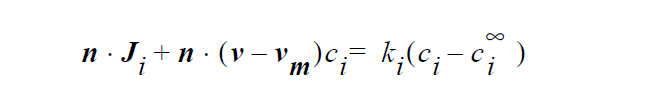
where n is the unit vector normal to the boundary, \(J_i\) is mass flux of species i, v is the fluid velocity, \(v_m\) is the mesh displacement velocity, \(k_i\) is mass transfer coefficient of species i, \(c_i\) is concentration of species i at the boundary surface, \(c_i^\infty\) and is reference concentration of species i. The units of \(J_i\), \(k_i\), \(c_i\) and \(c_i^\infty\) depend on the user’s choice. For example, if \(c_i\) and \(c_i^\infty\) are chosen to have units of moles/ \(cm^3\), then \(k_i\) has the unit of cm/ s, and \(J_i\) has the units of moles/ \(cm^2\) /s.
For the KIN_LEAK and VNORM_LEAK cards, the information from YFLUX boundary conditions corresponding to each species is needed. Goma automatically searches for these boundary conditions and uses an extra variable in the BC data storage to record the boundary condition number of the next YFLUX condition in a linked list; when the extra storage value is -1, there are no more YFLUX conditions at this boundary.
FAQs#
A question was raised regarding the use of volume flux in Goma; the following portion of the question and response elucidate this topic and the subject of units. Note the references in the response are to the Version 2.0 Goma User’s Manual.
Question: … I know what you are calling volume flux is mass flux divided by density. The point I am trying to make is that the conservation equations in the books I am familiar with talk about mass, energy, momentum, and heat fluxes. Why do you not write your conservation equations in their naturally occurring form? If density just so happens to be common in all of the terms, then it will be obvious to the user that the problem does not depend on density. You get the same answer no matter whether you input rho=1.0 or rho=6.9834, provided of course this does not impact iterative convergence. This way, you write fluxes in terms of gradients with the transport properties (viscosity, thermal conductivity, diffusion coefficient, etc.) being in familiar units.
Answer: First let me state the only error in the manual that exists with regard to the convection-diffusion equation is the following:
\(J_t\) in the nomenclature table … should be described as a volume flux with units of L/t, i.e., \(D ⋅ \Delta_yi\) , where D is in \(L^2\) ⁄ t units.
Now, … this is actually stated correctly, as it states the \(J_i\) is a diffusion flux (without being specific); to be more specific here, we should say it is a “volume flux of species i.” So, in this case D is in L ⋅ L ⁄ t units, \(y_i\) is dimensionless and it is immaterial that (the mass conservation equation) is multiplied by density or not, as long as density is constant.
Now, in Goma we actually code it up EXACTLY as in the … (mass conservation equation), i.e., there are no densities anywhere for the FICKIAN diffusion model. For the HYDRO diffusion model, we actually compute a \(J_i\) ⁄ ρ in the code, and handle variable density changes through that p . In that case \(J_i\) as computed in Goma is a mass flux vector, not a volume flux vector, but by dividing it by p and sending it back up to the mass conservation equation it changes back into a volume flux. i. e., everything is the same.
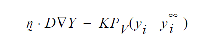
Concerning the units of the mass transfer coefficient on the YFLUX boundary condition, the above discussion now sets those. Goma clearly needs the flux in the following form:
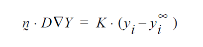
and dimensionally for the left hand side
where D is in units \(L^2\) /t , the gradient operator has units of 1/L so K HAS to be in units of L/t (period!) because \(y_i\) is a fraction.
So, if you want a formulation as follows:
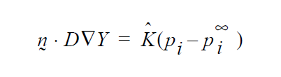
then K’s units will have to accommodate for the relationship between \(p_i\) and \(y_i\) in the liquid, hopefully a linear one as in Raoult’s law, i.e. if \(p_i\) = \(P_V\)\(y_i\) where \(P_v\) is the vapor pressure, then
and so K on the YFLUX command has to be \(KP_v\) ….and so on.
Finally, you will note, since we do not multiply through by density, you will have to take care of that, i. e., in the Price paper he gives K in units of t/L. So, that must be converted as follows:
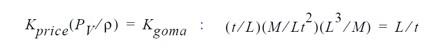
This checks out!
References#
Price, P. E., Jr., S. Wang, I. H. Romdhane, 1997. “Extracting Effective Diffusion Parameters from Drying Experiments”, AIChE Journal, 43, 8, 1925-1934.
YFLUX_CONST#
BC = YFLUX_CONST SS <bc_id> <integer> <float>
Description / Usage#
(WIC/MASS)
This boundary condition card is used to specify a constant diffusive mass flux of a given species. This flux quantity can be specified on a per mass basis (e.g. with units of g/ \(cm^2\) /s) or on a per mole basis (e.g. with units of moles/ \(cm^2\) /s), depending on the user’s choice of units in the species unknown.
Definitions of the input parameters are as follows:
YFLUX_CONST |
Name of the boundary condition (<bc_name>). |
SS |
Type of boundary condition (<bc_type>), where SS denotes side set in the EXODUS II database. |
<bc_id> |
The boundary flag identifier, an integer associated with <bc_type> that identifies the boundary location (side set in EXODUS II) in the problem domain. |
<integer> |
Species number. |
<float> |
Value of diffusive mass flux; the units of this quantity depends on the user’s choice of units for species concentration. |
Examples#
Following is a sample card:
BC = YFLUX_CONST SS 1 0 10000.2
Technical Discussion#
No Discussion.
References#
No References.
YFLUX_EQUIL#
BC = YFLUX_EQUIL SS <bc_id> {char_string} <integer> <float_list>
Description / Usage#
(WIC/MASS)
This boundary card is used when equilibrium-based mass transfer is occurring at an vapor-liquid external boundary; i.e.,
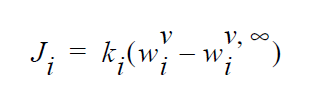
This is different from an internal boundary since only one phase is represented in the computational domain. This boundary condition then describes the rate of mass entering or leaving the boundary via vapor-liquid equilibria. The \(w_i^v\) is the mass fraction of component i in \(\underline{vapor}\) that is in equilibrium with the liquid phase. The \(w_i^{v \infty}\) is the bulk concentration of component i in vapor.
The <float_list> requires three input values; definitions of the input parameters are as follows:
YFLUX_EQUIL |
Name of the boundary condition. |
SS |
Type of boundary condition (<bc_type>), where SS denotes side set in the EXODUS II database. |
<bc_id> |
The boundary flag identifier, an integer associated with <bc_type> that identifies the boundary location (side set in EXODUS II) in the problem domain. |
{char_string} |
This refers to the equilibrium model for mass transfer; the options are either FLORY or RAOULT. |
<integer1> |
Species id. |
<float1> |
Total system pressure. |
<float2> |
Mass transfer coefficient. |
<float3> |
Bulk concentration in vapor ( \(w_i^{v \infty}\) ) |
Examples#
The following is a sample input card:
BC = YFLUX_EQUIL SS 1 FLORY 0 1. 5.4e-3 0.
Technical Discussion#
This boundary condition is very similar to VL_EQUIL and VL_POLY except that it is only applied at an external boundary where vapor phase is not modeled in the problem.
References#
GTM-007.1: New Multicomponent Vapor-Liquid Equilibrium Capabilities in GOMA, December 10, 1998, A. C. Sun
YFLUX_SULFIDATION#
BC = YFLUX_SULFIDATION SS <bc_id> {char_string} <integer> <float_list>
Description / Usage#
(WIC/MASS)
The YFLUX_SULFIDATION card enables computation of the molar flux of the diffusing species (e.g. copper vacancy) using copper-sulfidation kinetics at the specified boundary (gas/ \(Cu^2S\) or Cu/ \(Cu^2S\) interface). When used in conjunction with the KIN_LEAK card, it also enables the determination of velocity normal to the moving gas/ \(Cu^2S\) interface.
The <float_list> contains ten values to be defined; these and all input parameter definitions are as follows:
YFLUX_SULFIDATION |
Name of the boundary condition (<bc_name>). |
SS |
Type of boundary condition (<bc_type>), where SS denotes side set in the EXODUS II database. |
<bc_id> |
The boundary flag identifier, an integer associated with <bc_type> that identifies the boundary location (side set in EXODUS II) in the problem domain. |
{char_string} |
Name of sulfidation kinetic models. Allowable names are:
Detailed description of kinetic models with these name key words are presented in the Technical Discussion section below. |
<integer> |
Species number of concentration. |
<float1> |
Stoichiometric coefficient. |
<float2> |
Rate constant for forward copper sulfidation reaction. |
<float3> |
Activation energy for forward copper sulfidation reaction. |
<float4> |
Rate constant for backward copper sulfidation reaction. |
<float5> |
Activation energy for backward copper sulfidation reaction. |
<float6> |
Temperature. |
<float7> |
Bulk concentration of \(H^2S\) |
<float8> |
Bulk concentration of \(O^2\) |
<float9> |
Molecular weight of copper sulfide ( \(Cu_2S\) ) |
Examples#
Examples of this input card follow:
BC = YFLUX_SULFIDATION SS 3 SOLID_DIFFUSION_ELECTRONEUTRALITY 0 -2.0
1.46e+7 6300.0 1.2e+14 6300.0 303.0 1.61e-11 8.4e-6 159.14 5.6
BC = YFLUX_SULFIDATION SS 1 ANNIHILATION_ELECTRONEUTRALITY 0 1.0   10.0
0.0   0.0   0.0   303.0 1.61e-11 8.4e-6 159.14 5.6
BC = YFLUX_SULFIDATION SS 3 SOLID_DIFFUSION 1 -2.0 1.46e7 6300.0 1.2e+14
6300.0 303.0 1.61e-11 8.4e-6 159.14 5.6
BC = YFLUX_SULFIDATION SS 1 ANNIHILATION 1 1.0 10.0   0.0   0.0   0.0
303.0 1.61e-11 8.4e-6 159.14 5.6
Technical Discussion#
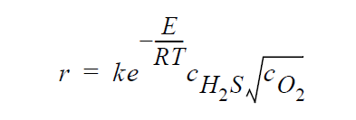
Key word SOLID_DIFFUSION_SIMPLIFIED refers to the following simplified kinetic model of copper sulfidation in which gas-phase diffusion is neglected and Cu is taken to be the diffusing species:
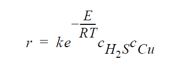
where r is molar rate of formation of sulfidation-corrosion product, \(Cu^2S\), per unit area, \(^cH_2S\) is the molar concentration of \(H_2S\) taken to be fixed at its bulk value, \(^cCu\) is the molar concentration of Cu at the sulfidation surface ( \(Cu_2S\) /gas interface), k is the rate constant, E is the activation energy, R is the universal gas constant, and T is the temperature.
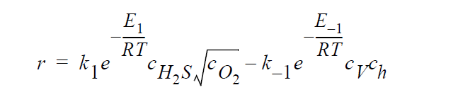
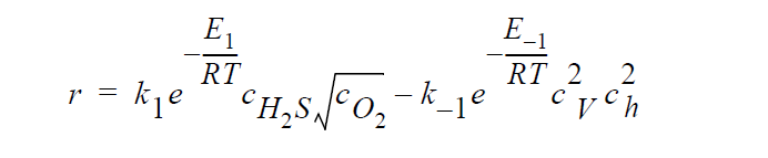
Key word SOLID_DIFFUSION refers to the following kinetic model of copper sulfidation in which gas-phase diffusion is neglected and Cu vacancies and electron holes are taken as the diffusing species:
where r is molar rate of formation of \(Cu_2S\) per unit area, \(^cH_2S\) and \(^cO_2\) are the molar concentrations of \(H_2S\) and \(O_2\), respectively, taken to be fixed at their bulk values, \(^c_V\) and \(^c_h\) are the molar concentrations of Cu vacancies and electron holes, respectively, at the sulfidation surface, \(k_1\) and \(k_{-1}\) are rate constants, respectively, for the forward and backward sulfidation reactions, \(E_1\) and \(E_{-1}\) are activation energies, respectively, for the forward and the backward sulfidation reactions.
Key word SOLID_DIFFUSION_ELECTRONEUTRALITY refers to the following kinetic model of copper sulfidation in which Cu vacancies and electron holes are taken as the diffusing species and the electroneutrality approximation is applied such that concentrations of Cu vacancies and electron holes are equal to each other:
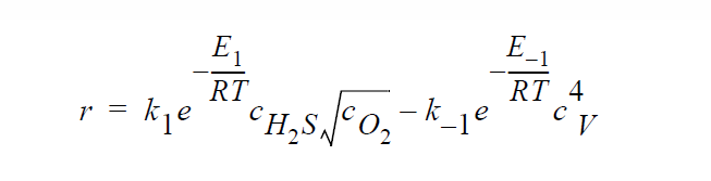
Key word SOLID_DIFFUSION_ELECTRONEUTRALITY_LINEAR refers to the following kinetic model of copper sulfidation:
Key word GAS_DIFFUSION refers to the following simplified kinetic model of copper sulfidation in which solid-phase diffusion is neglected, and \(H_2S\) and \(O_2\) are taken to be the diffusing species:
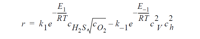
Key word FULL refers to the following kinetic model in which diffusion in both the gas phase and the solid phase are important, and \(H_2S\), \(O_2\), Cu vacancies, and electron holes are taken as the diffusing species:
where \(^cH_2S\) and \(^cO_2\) are the time-dependent molar concentrations of \(H_2S\) and \(O_2\), respectively, at the sulfidation surface.
Key word ANNIHILATION refers to the following kinetic model in which diffusion in both the gas phase and the solid phase are important, and \(H_2S\), \(O_2\), Cu vacancies, and electron holes are taken as the diffusing species:
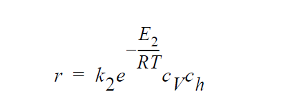
where \(k_2\) are \(E_2\) are the rate constant and activation energy, respectively, for the annihilation reaction.
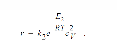
Key word ANNIHILATION_ELECTRONEUTRALITY is similar to ANNIHILATION except that, here, the electroneutrality approximation is applied and concentrations of Cu vacancies and electron holes are taken to be equal to each other:
YFLUX_SUS#
BC = YFLUX_SUS SS <bc_id> <integer>
Description / Usage#
(WIC/MASS)
This boundary defines a flux of suspension particles at an interface. Definitions of the input parameters are as follows:
YFLUX_SUS |
Name of the boundary condition (<bc_name>). |
SS |
Type of boundary condition (<bc_type>), where SS denotes side set in the EXODUS II database. |
<bc_id> |
The boundary flag identifier, an integer associated with <bc_type> that identifies the boundary location (side set in EXODUS II) in the problem domain. |
<integer> |
Species id; the species number for suspension particles. |
Examples#
The following is a sample input card:
BC = YFLUX_SUS SS 1 0
Technical Discussion#
This condition is only used in conjunction with the SUSPENSION liquid constitutive models, HYDRODYNAMIC diffusivity model, and SUSPENSION or SUSPENSION_PM density models. A theoretical outflux condition associated with suspension particles leaving the domain is tied to the Phillips diffusive-flux model. Please refer to discussions on HYDRODYNAMIC diffusivity to gain more understanding of the suspension flux model.
YFLUX_BV#
BC = YFLUX_BV SS <bc_id> <integer1> <floatlist>
Description / Usage#
(WIC/MASS)
The YFLUX_BV card enables computation of the molar flux of the specified species using Butler-Volmer kinetics at the specified boundary (namely, the electrode surface). When used in conjunction with the KIN_LEAK card, it also enables the determination of velocity normal to the moving solid-electrode surface.
The <floatlist> consists of nine values; definitions of the input parameters are as follows:
YFLUX_BV |
Name of the boundary condition (<bc_name>). |
SS |
Type of boundary condition (<bc_type>), where SS denotes side set in the EXODUS II database. |
<bc_id> |
The boundary flag identifier, an integer associated with <bc_type> that identifies the boundary location (side set in EXODUS II) in the problem domain. |
<integer1> |
Species number of concentration. |
<float1> |
Stoichiometric coefficient. |
<float2> |
Kinetic rate constant. |
<float3> |
Reaction order. |
<float4> |
Anodic direction transfer coefficient. |
<float5> |
Cathodic direction transfer coefficient. |
<float6> |
Electrode potential or applied voltage. |
<float7> |
Theoretical open-circuit potential. |
<float8> |
Molecular weight of solid deposit. |
<float9> |
Density of solid deposit. |
Examples#
The following is a sample input card:
BC = YFLUX_BV SS 1 0 -1. 0.00001 1. 0.21 0.21 -0.8 -0.22 58.71 8.9
Technical Discussion#
No Discussion.
YFLUX_HOR#
BC = YFLUX_HOR SS <bc_id> <integer> <floatlist>
Description / Usage#
(WIC/MASS)
The YFLUX_HOR card enables computation of the molar flux of the specified species at the specified boundary (i.e., at the electrode surface) using the linearized Butler- Volmer kinetics such as that for the hydrogen-oxidation reaction in polymerelectrolyte- membrane fuel cells.
The <floatlist> consists of 10 values; definitions of the input parameters are as follows:
YFLUX_HOR |
Name of the boundary condition (<bc_name>). |
SS |
Type of boundary condition (<bc_type>), where SS denotes side set in the EXODUS II database. |
<bc_id> |
The boundary flag identifier, an integer associated with <bc_type> that identifies the boundary location (side set in EXODUS II) in the problem domain. |
<integer> |
Species number of concentration. |
<float1> |
Product of interfacial area per unit volume by exchange current density, \(ai_0\), in units of \(A/cm^3\). |
<float2> |
Catalyst layer or catalyzed electrode thickness, H, in unit of cm. |
<float3> |
Reference concentration, \(c_{ref}\), in units of moles/ \(cm^3\). |
<float4> |
Anodic direction transfer coefficient, \(\alpha_a\). |
<float5> |
Cathodic direction transfer coefficient, \(\alpha_c\). |
<float6> |
Temperature, T, in unit of K. |
<float7> |
Theoretical open-circuit potential, \(U_0\), in unit of V. |
<float8> |
Reaction order, \(\beta\). |
<float9> |
Number of electrons involved in the reaction, n. |
<float10> |
Electrode potential, V, in unit of V. |
Examples#
The following is a sample input card:
BC = YFLUX_HOR SS 14 0 1000. 0.001 4.e-5 1. 1. 353. 0. 0.5 2. 0.
Technical Discussion#
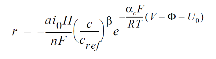
For electrochemical reactions such as the hydrogen-oxidation reaction (HOR), surface overpotential is relatively small such that the Butler-Volmer kinetic model can be linearized to yield:
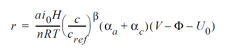
where r is the surface reaction rate in units of moles/ \(cm^2-s\); \(ai_0\) denotes the product of interfacial area per unit volume by exchange current density, which has units of \(A/cm^3\); H is the catalyst layer or catalyzed electrode thickness in unit of cm; n is the number of electrons involved in the electrochemical reaction; R is the universal gas constant ( \(\equiv\) 8.314 J/mole-K); T is temperature in unit of K; c and \(c_{ref}\) are, respectively, species and reference molar concentrations in units of moles/ \(cm^3\); \(\beta\) is reaction order; \(\alpha_a\) and \(\alpha_c\) are, respetively, the anodic and cathodic transfer coefficients; V and \(\phi\) are, respectively, the electrode and electrolyte potentials in unit of V; \(U_0\) and is the opencircuit potential in unit of V.
References#
Newman, Electrochemical Systems, 2nd Edition, Prentice-Hall, NJ (1991).
K. S. Chen and M. A. Hickner, “Modeling PEM fuel cell performance using the finiteelement method and a fully-coupled implicit solution scheme via Newton’s technique”, in ASME Proceedings of FUELCELL2006-97032 (2006).
YFLUX_ORR#
BC = YFLUX_ORR SS <bc_id> <integer> <floatlist>
Description / Usage#
(WIC/MASS)
The YFLUX_ORR card enables computation of the molar flux of the specified species at the specified boundary (i.e., at the electrode surface) using the Tafel kinetics such as that for the oxygen-reduction reaction in polymer-electrolyte-membrane fuel cells.
The <floatlist> consists of 9 values; definitions of the input parameters are as follows:
YFLUX_ORR |
Name of the boundary condition (<bc_name>). |
SS |
Type of boundary condition (<bc_type>), where SS denotes side set in the EXODUS II database. |
<bc_id> |
The boundary flag identifier, an integer associated with <bc_type> that identifies the boundary location (side set in EXODUS II) in the problem domain. |
<integer> |
Species number of concentration. |
<float1> |
Product of interfacial area per unit volume by exchange current density, \(ai_0\), in units of \(A/cm^3\). |
<float2> |
Catalyst layer or catalyzed electrode thickness, H, in unit of cm. |
<float3> |
Reference concentration, \(c_{ref}\), in units of moles/ \(cm^3\). |
<float4> |
Cathodic direction transfer coefficient, \(\alpha_c\). |
<float5> |
Temperature, T, in unit of K. |
<float6> |
Electrode potential, V, in unit of V. |
<float7> |
Theoretical open-circuit potential, \(U_0\), in unit of V. |
<float8> |
Reaction order, \(\beta\). |
<float9> |
Number of electrons involved in the reaction, n. |
Examples#
The following is a sample input card:
BC = YFLUX_ORR SS 15 1 0.01 0.001 4.e-5 1. 353. 0.7 1.18 1. 4.
Technical Discussion#
For electrochemical reactions such as the hydrogen-oxidation reaction (HOR), surface overpotential is relatively small such that the Butler-Volmer kinetic model can be linearized to yield:
where r is the surface reaction rate in units of moles/ \(cm^2-s\); \(ai_0\) denotes the product of interfacial area per unit volume by exchange current density, which has units of A/ \(cm^3\); H is the catalyst layer or catalyzed electrode thickness in unit of cm; n is the number of electrons involved in the electrochemical reaction; F is the Faraday’s constant ( \(\equiv\) 96487 C/mole); c and \(c_{ref}\) are, respectively, species and reference molar concentrations in units of moles/ \(cm^3\); \(\beta\) is reaction order; \(\alpha_c\) is the anodic and cathodic transfer coefficient; R is the universal gas constant ( \(\equiv\) 8.314 J/mole-K); T is temperature in unit of K; V and \(\phi\) are, respectively, the electrode and electrolyte potentials in unit of V; \(U_0\) and is the open-circuit potential in unit of V.
References#
Newman, Electrochemical Systems, 2nd Edition, Prentice-Hall, NJ (1991).
K. S. Chen and M. A. Hickner, “Modeling PEM fuel cell performance using the finiteelement method and a fully-coupled implicit solution scheme via Newton’s technique”, in ASME Proceedings of FUELCELL2006-97032 (2006).
YFLUX_USER#
BC = YFLUX_USER SS <bc_id> <integer> <float_list>
Description / Usage#
(WIC/MASS)
This boundary condition card is used to set mass flux to a user-prescribed function and integrate by parts again. The user should provide detailed flux conditions in the mass_flux_user_surf routine in user_bc.c. The flux quantity is specified on a per mass basis so the heat and mass transfer coefficients are in units of L/t.
Definitions of the input parameters are as follows:
YFLUX_USER |
Name of the boundary condition (<bc_name>). |
SS |
Type of boundary condition (<bc_type>), where SS denotes side set in the EXODUS II database. |
<bc_id> |
The boundary flag identifier, an integer associated with <bc_type> that identifies the boundary location (side set in EXODUS II) in the problem domain. |
<integer> |
Species number of concentration. |
<float_list> |
A list of float values separated by spaces which will be passed to the user-defined subroutines so the user can vary the parameters of the boundary condition. This list of float values is passed as a one-dimensional double array to the appropriate C function. |
Examples#
The following is a sample input card:
BC = YFLUX_USER SS 2 0 .5 .5
Technical Discussion#
No Discussion.
References#
No References.
YFLUX_ALLOY#
BC = YFLUX_ALLOY SS <bc_id> <integer1> <float_list>
Description / Usage#
(WIC/MASS)
This boundary condition card calculates the surface integral for a mass flux transfer model for the evaporation rate of molten metal.
The <float_list> requires six values; definitions of the input parameters are as follows:
YFLUX_ALLOY |
Name of the boundary condition (<bc_name>). |
SS |
Type of boundary condition (<bc_type>), where SS denotes side set in the EXODUS II database. |
<bc_id> |
The boundary flag identifier, an integer associated with <bc_type> that identifies the boundary location (side set in EXODUS II) in the problem domain. |
<integer1> |
Species number. |
<float1> |
Liquidus temperature of metal alloy, \(T_m\). |
<float2> |
Base Concentration, \(y^\infty\). |
<float3> |
Coefficient \(c_0\). |
<float4> |
Coefficient \(c_1\). |
<float5> |
Coefficient \(c_2\). |
<float6> |
Coefficient \(c_3\). |
Examples#
The following is a sample input card:
BC = YFLUX_ALLOY SS 10 0 1623.0 0.5 0.01 -1e-3 1e-4 -1e-5
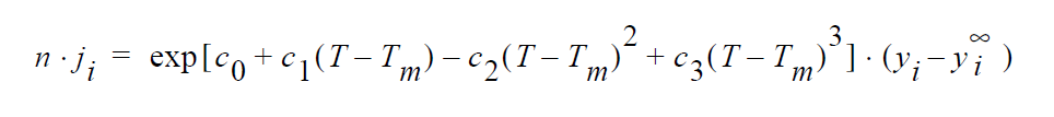
Technical Discussion#
Basically the difference between this model and the simple convective mass transfer coefficient (say \(k_i\) for YFLUX) is that the transfer coefficient here (the exponential term) has a cubic dependence on temperature.
YTOTALFLUX_CONST#
BC = YTOTALFLUX_CONST SS <bc_id> <integer> <float>
Description / Usage#
(WIC/MASS)
This boundary condition card is used to specify a constant total mass flux (including contribution from diffusion, migration, and convection) of a given species. This card enables the treatment of the situation in which diffusion, migration and convection fluxes cancel each other such that the total flux vanishes (e.g. is equal to zero). This flux quantity can be specified on a per mass basis (i.e., with units of g/ \(cm^2\)/s) or on a per mole basis (e.g. with units of moles/\(cm^2\)/s), depending on the user’s choice of units in the species concentration unknown.
Definitions of the input parameters are as follows:
YTOTALFLUX_CONST |
Name of the boundary condition (<bc_name>). |
SS |
Type of boundary condition (<bc_type>), where SS denotes side set in the EXODUS II database. |
<bc_id> |
The boundary flag identifier, an integer associated with <bc_type> that identifies the boundary location (side set in EXODUS II) in the problem domain. |
<integer> |
Species number of concentration. |
<float> |
Value of total mass flux - the units of this quantity depends on the user’s choice of units for species concentration. |
Examples#
Following is a sample card:
BC = YTOTALFLUX_CONST SS 5 0 0.0
Technical Discussion#
No Discussion.
VL_EQUIL#
BC = VL_EQUIL SS <bc_id> <integer_list> <float_list>
Description / Usage#
(SIC/MASS)
This boundary condition card enforces vapor-liquid equilibrium between a gas phase and a liquid phase using Raoult’s law. The condition only applies to interphase mass, heat, and momentum transfer problems with discontinuous (or multivalued) variables at an interface, and it must be invoked on fields that employ the Q1_D or Q2_D interpolation functions to “tie” together or constrain the extra degrees of freedom at the interface in question.
The <integer_list> has three values and the <float_list> has five values; definitions of the input parameters are as follows:
VL_EQUIL |
Name of the boundary condition (<bc_name>). |
SS |
Type of boundary condition (<bc_type>), where SS denotes side set in the EXODUS II database. |
<bc_id> |
The boundary flag identifier, an integer associated with <bc_type> that identifies the boundary location (side set in EXODUS II) in the problem domain. |
<integer1> |
Species number. |
<integer2> |
Element block ID of liquid phase. |
<integer3> |
Element block ID of gas phase. |
<float1> |
Base ambient pressure in gas phase. |
<float2> |
Molecular weight of first volatile species. |
<float3> |
Molecular weight of second volatile species. |
<float4> |
Molecular weight of condensed phase. |
<float5> |
Molecular weight of insoluble gas phase. |
This boundary condition is applied to ternary, two-phase flows that have rapid mass exchange between phases, rapid enough to induce a diffusion velocity at the interface, and to thermal contact resistance type problems. The best example of this is rapid evaporation of a liquid component into a gas. In the current discontinuous mass transfer model, we must require the same number of components on either side of interface. In this particular boundary, two of three components are considered volatile, so they participate in both vapor and liquid phases. The third component is considered either non-volatile or non-condensable, so it remains in a single phase.
Examples#
A sample input card follows for this boundary condition:
BC = VL_EQUIL SS 4 0 1 2 1.e+06 28. 18. 1800. 18.
The above card demonstrates these characteristics: species number is “0”; liquid phase block id is 1; gas phase block id is 2; ambient pressure is 1.e6 Pa; the molecular weights of the volatile species are 28 and 18; of the condensed phase and insoluble portion of the gas phase, 1800 and 18, respectively.
Technical Discussion#
One of the simplest forms of the equilibrium relation is the Raoult’s law, where the mole fraction of a species is equal to its mole fraction in the liquid multiplied by the ratio of its pure component vapor pressure to the total pressure in the system.
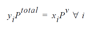
where \(y_i\) are the mole fraction of species i in the gas phase and \(x_i\) is the mole fraction in the liquid phase. The molecular weights required in this boundary card are used for converting mass fractions to mole fractions. The temperature dependency in the equilibrium expression comes from a temperature-dependent vapor pressure model. Either Riedel or Antoine temperature-dependent vapor pressure model can be specified in the VAPOR PRESSURE material card in order to link temperature to Raoult’s law.
References#
GTM-007.1: New Multicomponent Vapor-Liquid Equilibrium Capabilities in GOMA, December 10, 1998, A. C. Sun
Schunk, P.R. and Rao, R.R. 1994. “Finite element analysis of multicomponent twophase flows with interphase mass and momentum transport,” IJNMF, 18, 821-842.
VL_POLY#
BC = VL_POLY SS <bc_id> {char_string} <integer_list> <float>
Description / Usage#
(SIC/MASS)
This boundary condition card enforces vapor-liquid equilibrium between a gas phase and a liquid phase using Flory-Huggins activity expression to describe polymer-solvent mixtures. The condition only applies to interphase mass, heat, and momentum transfer problems with discontinuous (or multivalued) variables at an interface, and it must be invoked on fields that employ the Q1_D or Q2_D interpolation functions to “tie” together or constrain the extra degrees of freedom at the interface in question.
There are three input values in the <integer_list>; definitions of the input parameters are as follows:
VL_POLY |
Name of the boundary condition (<bc_name>). |
SS |
Type of boundary condition (<bc_type>), where SS denotes side set in the EXODUS II database. |
<bc_id> |
The boundary flag identifier, an integer associated with <bc_type> that identifies the boundary location (side set in EXODUS II) in the problem domain. |
{char_string} |
the concentration basis; two options exist:
|
<integer1> |
Species number of concentration. |
<integer2> |
Element block id that identifies the liquid phase. |
<integer3> |
Element block id that identifies the vapor phase. |
<float> |
Total pressure of the system. |
Examples#
This is a sample input card for this boundary condition:
BC = VL_POLY SS 7 MASS 0 1 2 1.e+05
Technical Discussion#
One of the simplest forms of the equilibrium relation is the Raoult’s law, where the mole fraction of a species is equal to its mole fraction in the liquid multiplied by the ratio of its pure component vapor pressure to the total pressure in the system.
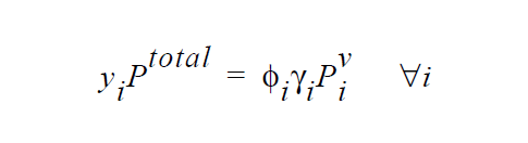
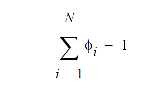
\(\gamma_i\) is defined as the activity coefficient of species i and is considered a departure function from the Raoult’s law. The fugacity in the liquid is reformulated in terms of volume fraction \(\phi_i\) for polymer mixtures to avoid referencing the molecular weight of polymer (Patterson, et. al., 1971).
Based on an energetic analysis of excluded volume imposed by the polymer, the activity coefficient model of Flory-Huggins is widely used for polymer-solvent mixtures (Flory, 1953). The general form of the Flory-Huggins model for multicomponent mixtures is a summation of binary interactions terms; i.e.,
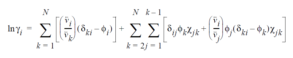
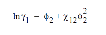
\(v_i\) is the molar volume of component i (or the average-number molar volume if i is a polymer). \(\zeta_{ki}\) is the Dirac delta. \(\chi_{jk}\) is known as the Flory-Huggins interaction parameter between components j and k, and is obtainable by fitting the solubility data to the above model. For a simple binary pair (solvent (1)-polymer (2)) and assuming \(v_2\) » \(v_1\), the above model reduces to a simpler form.
References#
Flory, P., Principles of Polymer Chemistry, Cornell University Press, New York (1953)
Patterson, D., Y.B. Tewari, H.P. Schreiber, and J.E. Guillet, “Application of Gas-Liquid Chromatography to the Thermodynamics of Polymer Solutions,”Macromolecules, 4, 3, 356-358 (1971)
GTM-007.1: New Multicomponent Vapor-Liquid Equilibrium Capabilities in GOMA, December 10, 1998, A. C. Sun
VL_EQUIL_PSEUDORXN#
BC = VL_EQUIL_PSEUDORXN SS <bc_id> <integer_list> <float>
Description / Usage#
(WIC/MASS)
This boundary condition card enforces vapor-liquid equilibrium between a gas phase and a liquid phase species component using Raoult’s law expressed via a finite-rate kinetics formalism. The condition only applies to problems containing internal interfaces with discontinuous (or multilevel) species unknown variables. The species unknown variable must employ the Q1_D or Q2_D interpolation functions in both adjacent element blocks. This boundary condition constrains the species equations on both sides of the interface (i.e., supplies a boundary condition) by specifying the interfacial mass flux on both sides.
Definitions of the input parameters are as follows:
VL_EQUIL_PSEUDORXN |
Name of the boundary condition (<bc_name>). |
SS |
Type of boundary condition (<bc_type>), where SS denotes side set in the EXODUS II database. |
<bc_id> |
The boundary flag identifier, an integer associated with <bc_type> that identifies the boundary location (side set in EXODUS II) in the problem domain. |
<integer1> |
Species number. |
<integer2> |
Element Block ID of the liquid phase. |
<integer3> |
Element Block ID of the gas phase. |
<float> |
Rate constant for the forward reaction in units of length divided by time. |
This boundary condition is typically applied to multicomponent two-phase flows that have rapid mass exchange between phases. The best example of this is rapid evaporation of a liquid component into a gas.
Examples#
The following sample input card
BC = VL_EQUIL_PSEUDORXN SS 4 0 1 2 100.
demonstrates the following characteristics: species number is “0”; liquid phase element block id is “1”; gas phase element block id is “2”; a forward rate constant of 100.0 cm \(s^{-1}\).
Technical Discussion#
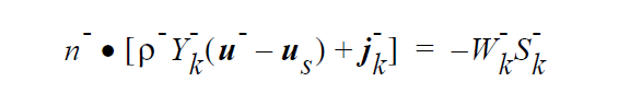
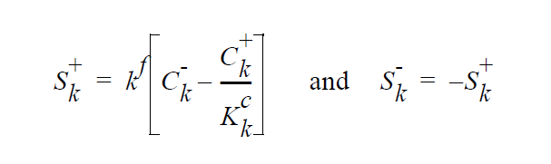
The VL_EQUIL_PSEUDORXN boundary condition uses the following equations representing a kinetic approach to equilibrium expressed by Raoult’s law, relating species k on the liquid side to species k on the gas side.
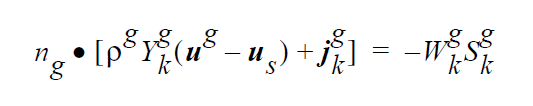
where
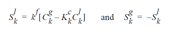
and where
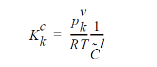
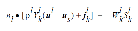
The usage of the same index, k, on either side of the interface is deliberate and represents a stoichiometric limitation to this type of boundary condition. \(Y_k^l\) and \(Y_k^g\) are the mass fraction of species k on the liquid and gas sides of the interface, respectively. \(W_k^l\) is the molecular weight of species k. \(S_k^l\) is the source term for creation of species k in the liquid phase at the interface (mol \(cm^{-2}\) \(s^{-1}\) ). is the pseudo reaction rate ( \(cm s^{-1}\) ) input from the boundary condition card. \(K_k^c\) is the concentration equilibrium constant, which for the restricted stoichiometry cases covered by this boundary condition, is unitless. \(p_k^v\) is the vapor pressure of gas species k above a liquid entirely consisting of liquid species k. It is a function of temperature. \(\tilde{C}_l\) is the average concentration in the liquid (mol \(cm^{-3}\)). \(C_k^l\) and \(C_k^g\) are the liquid and gas concentrations of species k (mol \(cm^{-3}\)).
The choice for the independent variable is arbitrary, although it does change the actual equation formulation for the residual and Jacobian terms arising from the boundary condition. The internal variable Species_Var_Type in the Uniform_Problem_Description structure may be queried to determine what the actual species independent variable is. Also note, if mole fractions or molar concentration are chosen as the independent variable in the problem, the convention has been to formulate terms of the residuals in units of moles, cm, and seconds. Therefore, division of the equilibrium equations by \(W_k\) would occur before their inclusion into the residual. \(j_k^l\) and \(j_k^g\) are the diffusive flux of species k (gm \(cm^{-2}\) \(s^{-1}\) ) relative to the mass averaged velocity. \(u_s\) is the velocity of the interface. A typical value of \(k^f\) that would lead to good numerical behavior would be 100 cm \(s^{-1}\), equivalent to a reaction with a reactive sticking coefficient of 0.01 at 1 atm and 300 K for a molecule whose molecular weight is near to \(N_2\) or \(H_2S\).
IS_EQUIL_PSEUDORXN#
BC = IS_EQUIL_PSEUDORXN SS <bc_id> <integer_list> <float>
Description / Usage#
(WIC/MASS)
This boundary condition card enforces equilibrium between a species component in two ideal solution phases via a finite-rate kinetics formalism. The condition only applies to problems containing internal interfaces with discontinuous (or multilevel) species unknown variables. The species unknown variable must employ the Q1_D or Q2_D interpolation functions in both adjacent element blocks. This boundary condition constrains the species equations on both sides of the interface (i.e., supplies a boundary condition) by specifying the interfacial mass flux on both sides.
IS_EQUIL_PSEUDORXN is equivalent to the VL_EQUIL_PSEUDORXN except for the fact that we do not assume that one side of the interface is a gas and the other is a liquid. Instead, we assume that both materials on either side of the interface are ideal solutions, then proceed to formulate an equilibrium expression consistent with that.
The <integer_list> requires three values; definitions of the input parameters are as follows:
IS_EQUIL_PSEUDORXN |
Name of the boundary condition (<bc_name>). |
SS |
Type of boundary condition (<bc_type>), where SS denotes side set in the EXODUS II database. |
<bc_id> |
The boundary flag identifier, an integer associated with <bc_type> that identifies the boundary location (side set in EXODUS II) in the problem domain. |
<integer1> |
Species number. |
<integer2> |
Element Block ID of the first phase, the “+” phase. |
<integer3> |
Element Block ID of the second phase, the “-” phase. |
<float> |
Rate constant for the forward reaction in units of length divided by time. |
Examples#
The sample card:
BC = IS_EQUIL_PSEUDORXN SS 4 0 1 2 100.
demonstrates the following characteristics: species number is “0”; the “+” phase element block id is “1”; the “-” phase element block id is “2”; a forward rate constant of 100. cm \(s^{-1}\).
Technical Discussion#
The IS_EQUIL_PSEUDORXN boundary condition uses the following equations representing a kinetic approach to equilibrium expressed by an ideal solution model for thermodynamics on either side of the interface. Initially, we relate species k on the + side to species k on the - side of the interface via a kinetic formulation, whose rate constant is fast enough to ensure equilibrium in practice. However, later we may extend the capability to more complicated stoichiometric formulations for equilibrium, since the formulation for the equilibrium expression is readily extensible, unlike Goma’s previous treatment.
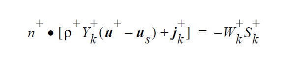
where
The “-” phase is defined as the reactants, while the “+” phase is defined to be the products. The expression for the concentration equilibrium constant, \(K_k^c\) , is based on the ideal solution expression for the chemical potentials for species k in the two phases [Denbigh, p. 249],
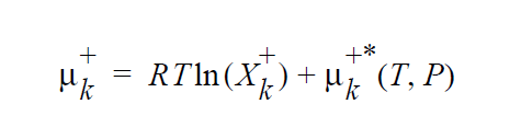
where \(\mu_k^{+*}\) (T,P) is defined as the chemical potential of species k in its pure state (or a hypothetical pure state if a real pure state doesn’t exist) at temperature T and pressure P. \(\mu_k^{+*}\) (T,P) is related to the standard state of species k in phase +, \(\mu_k^+\), \(\underline{o}\) + (T) , which is independent of pressure, through specification of the pressure dependence of the pure species k. Two pressure dependencies are initially supported:


With these definitions, \(K_k^c\) can be seen to be equal to
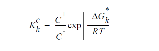
where

The chemical potential for a species in a phase will be calculated either from CHEMKIN or from the Chemical Potential, Pure Species Chemical Potential, and Standard State Chemical Potential cards in the materials database file.
The choice for the independent variable for the species unknown is relatively arbitrary,although it does change the actual equation formulation for the residual and Jacobian terms arising from the boundary condition. The internal variable Species_Var_Type in the Uniform_Problem_Description structure is queried to determine what the actual species independent variable is. A choice of SPECIES_UNDEFINED_FORM is unacceptable. If either mole fractions or molar concentration is chosen as the independent variable in the problem, the convention has been to formulate terms of the residuals in units of moles, cm, and seconds. Therefore, division of the equilibrium equations \(W_k\) by occurs before their inclusion into the residual. \(J^l_k\) and \(J^g_k\) are the diffusive flux of species k ( gm \(cm^{-2}\) \(s^{-1}\) ) relative to the mass-averaged velocity. \(u^s\) is the velocity of the interface. A typical value of \(k^f\) that would lead to good numerical behavior would be 100 cm \(s^{-1}\), equivalent to a reaction with a reactive sticking coefficient of 0.01 at 1 atm and 300 K for a molecule whose molecular weight is near to \(N_2\) or \(H_2 S\).
References#
Denbigh, K., The Principles of Chemical Equilibrium, Cambridge University Press, Cambridge, 1981
SURFACE_CHARGE#
BC = SURFACE_CHARGE SS <bc_id> <integer> <float>
Description / Usage#
(SIC/MASS)
The SURFACE_CHARGE card specifies the electrostatic nature of a surface: electrically neutral, positively charged or negatively charged.
Definitions of the input parameters are as follows:
SURFACE_CHARGE |
Name of the boundary condition (<bc_name>). |
|
SS |
Type of boundary condition (<bc_type>), where SS denotes side set in the EXODUS II database. |
|
<bc_id> |
The boundary flag identifier, an integer associated with <bc_type> that identifies the boundary location (side set in EXODUS II) in the problem domain. |
|
<integer> |
Index of species to which surface charge condition applies. |
|
<float> |
z, value of surface charge. |
|
0 |
electroneutrality |
|
positive z |
positively charged surface |
|
negative z |
negatively charged surface |
|
Examples#
The following input card indicates that on side set 1 species 1 is electrically neutral:
BC = SURFACE_CHARGE SS 1 1 0.0
FLUIDITY_EQUILIBRIUM#
BC = FLUIDITY_EQUILIBRIUM SS <bc_id> <species index>
Description / Usage#
(SIC/MASS)
Definitions of the input parameters are as follows:
- FLUIDITY_EQUILIBRIUM
Name of the boundary condition
- SS
This is applied to a side set
- <bc_id>
The SS id where we apply this BC
- <species index>
The 0-based species index associated with the FLUIDITY source term
Examples#
Following are two sample cards:
BC = FLUIDITY_EQUILIBRIUM SS 2
Technical Discussion#
This replaces the boundary equations with the equivalent equation with \(\mathbf{u}\cdot\nabla c = 0\) replacing the advection term.