Category 2: Mesh Equations#

The boundary conditions in this section involve the mesh motion equations in LAGRANGIAN or ARBITRARY form (cf. Mesh Motion card). These conditions can be used to pin the mesh, specify its slope at some boundary intersection, apply a traction to a surface, etc. Several more boundary conditions that are applied to the mesh motion equations but include other problem physics are also available.

DISTNG#

BC = DISTNG SS <bc_id> <float>

Description / Usage#

(PCC/ROTATED MESH)

This boundary condition card is used to specify a distinguishing condition for mesh motion based on an isotherm, viz. the distinguishing condition forces the mesh boundary to which it is applied to take on a position such that the temperature is constant and at the specified value, all along the boundary. This condition causes the vector mesh motion equations (viz. mesh1, mesh2, and mesh3 on EQ cards) to be rotated into normal-tangential form. In two dimensions, this condition is applied to the normal component automatically; in three dimensions it is suggested to put it on the normal component, as specified by the ROT conditions. Definitions of the input parameters are as follows:

DISTNG	Name of the boundary condition (<bcname>).
SS	Type of boundary condition (<bc_type>), where SS denotes side set in the EXODUS II database.
<bc_id>	The boundary flag identifier, an integer associated with <bc_type> that identifies the boundary location (side set in EXODUS II) in the problem domain.
<float>	Value of temperature/isotherm. To apply a variable temperature, e.g., as a function of the concentration, it is suggested that the user-defined boundary conditions be used, like SPLINE or GEOM.

Examples#

The following is a sample input card:

BC = DISTNG SS 123 273.0

This card forces the boundary defined by EXODUS II side set number 123 to conform to the isotherm temperature of 273.0.

Technical Discussion#

The mathematical form of this distinguishing condition is as follows:

\[T - T_{\mathrm{mp}} = 0\]

where \(T_{\mathrm{mp}}\) is the specified temperature parameter. This condition has been used extensively for macroscale and microscale melting problems, whereby one needs to distinguish a molten region from a solidified or mushy region with liquidus and solidus temperatures. In three dimensions, usage needs to be completed with a companion ROT input card which directs the equation application of the condition.

FAQs#

Continuation Strategies for Free Surface Flows In free surface problems, there exists one or more boundaries or internal surfaces whose position(s) are unknown a priori. As such, the geometry of the problem becomes part of the problem and must be determined together with the internal physics. Most problems of this sort cannot be solved with a trivial initial guess to the solution vector, mainly because the conditions which determine the surface position are closely coupled to the active physics in the bulk. Thus, these problems require continuation (zero or higher order) to achieve a converged solution to a desired state. The continuation strategy typically involves turning on and off the conditions which distinguish the position of the free surface(s); one such strategy is described in this FAQ.

Distinguishing conditions in Goma serve two purposes: (1) they can be used to locate a surface whose position depends on internal and interfacial transport phenomena, and (2) they can be used to prescribe solid boundary position or motion. The first type of condition contains field variables needed to locate the interface or free surface position, and hence ties the mesh motion to the problem physics, i.e., mass, momentum, and energy transport phenomena. Currently, the side-set boundary conditions of type DISTNG, KINEMATIC, and KIN_LEAK fall into this class. The second type of condition requires only geometrical information from the mesh, and, although geometrically couples the mesh motion to the problem physics, it tends not to be so tightly coupled. Currently, boundary conditions PLANE, PLANEX, PLANEY, PLANEZ, SPLINE, SPLINEX, SPLINEY, and SPLINEZ fall into this class.

In two dimensions, there is no need to use PLANEX, PLANEY, PLANEZ, SPLINEX, SPLINEY, and SPLINEZ. Because the code automatically rotates the mesh residual equations and the corresponding Jacobian entries into normal-tangential form on the boundary, SPLINE, PLANE, and DISTNG are the only cards required to specify the position of the boundary. Currently, in three dimensions, the logic for the same rotation concept is not totally functional, and one must use the PLANEX, etc. cards to designate which component of the mesh stress residual equation receives the distinguishing conditions.

If cards DISTNG, KINEMATIC, and KIN_LEAK, i.e., distinguishing conditions of type 1, are absent in any simulation, then any initial guess for the transport field equations, i.e., energy and momentum, has a chance of converging, as long as the initial mesh displacement guess is within the radius of convergence of the mesh equations and associated boundary conditions. For example, if the side sets of the EXODUS II database mesh correspond somewhat closely to what is prescribed with PLANE and SPLINE-type conditions, then an initial guess of the NULL vector has a good chance of converging, so long as the velocities and temperatures are within “converging distance.”

When conditions from the first class are present, i.e., either DISTNG, KIN_LEAK or KINEMATIC, then the following procedure should be followed:

Set the keyword for the Initial Guess character_string to zero, one, or random.
Obtain a solution (run Goma) with the initial guess for the free surfaces distinguished as KINEMATIC (or other) coming from the EXODUS II database, but without the KINEMATIC (or other) card(s). That is, “fix” those surfaces with either a PLANE or SPLINE command, or simply place no distinguishing condition on them (this works only if the grid has not been previously “stressed”, i.e., all the displacements are zero). The rest of the “desired” physics should be maintained. If any surface is distinguished as KINEMATIC, then it is highly advantageous to place a VELO_NORMAL condition on that surface for startup, and set the corresponding floating point datum to zero. This effectively allows the fluid to “slip” along that boundary as if it were a shear free condition.
Set the keyword in the Initial Guess character_string to read.
Copy the file named in SOLN file into the file named in GUESS file.
Release the free boundaries by taking off any current distinguishing condition cards and adding the appropriate KINEMATIC (or other) card. Adjust all other boundary conditions appropriately.
Run Goma, using a relaxed Newton approach (factor less than unity but greater than zero - e.g., 0.1) for complex flows.

When dealing with material surface boundaries distinguished by the kinematic boundary condition, the nature of that condition requires a non-zero and substantial component of velocity tangent to the surface upon start-up. In this case, it can be advantageous to use the VELO_TANGENT card to set the velocity along the free surface to some appropriate value prior to releasing the free surface (in the third step above). Of course this card will be removed in subsequent steps. Also, although not necessary, a smooth, “kinkless”, initial guess to the free surface shape is helpful because it reduces the amount of relaxation required on the Newton iteration.

Obtaining start-up solutions of most coating flow configurations is still an art. The best way to start up a coating flow analysis may be to acquire a “template” developed from a previous analysis of some closely related flows.

References#

Allen Roach’s or Randy’s ESR tutorials. Perhaps these need to be put into the repository.

DXDYDZ#

BC = {DX | DY | DZ} NS <bc_id> <float1> [float2]

Description / Usage#

(DC/MESH)

This boundary condition format is used to set a constant X, Y, or Z displacement. Each such specification is made on a separate input card. These boundary conditions must be applied to node sets. Definitions of the input parameters are as follows:

{DX \| DY \| DZ}	Two-character boundary condition name (<bc_name>) that defines the displacement, where: DX - X displacement DY - Y displacement DZ - Z displacement
NS	Type of boundary condition (<bc_type>), where NS denotes node set in the EXODUS II database.
<bc_id>	The boundary flag identifier, an integer associated with <bc_type> that identifies the boundary location (node set in EXODUS II) in the problem domain.
<float1>	Value of the displacement (X, Y, or Z) defined above.
[float2]	An optional parameter (that serves as a flag to the code for a Dirichlet boundary condition). If a value is present, and is not -1.0, the condition is applied as a residual equation. Otherwise, it is a “hard set” condition and is eliminated from the matrix. The residual method must be used when this Dirichlet boundary condition is used as a parameter in automatic continuation sequences.

Examples#

Following is a sample card which applies an X-displacement boundary condition to the nodes in node set 100, specifically an X-Displacement of 1.0. These displacements are applied immediately to the unknowns and hence result in immediate mesh displacements from the initial state.

BC = DX NS 100   1.0

This sample card applies the same condition as above, except as a residual equation that is iterated upon with Newton’s method.

BC = DX NS 100 1.0   1.0

The second float 1.0 forces this application. This approach is advisable in most situations, as the nodes are gradually moved as a part of the mesh deformation process; sudden movements, as in the first example, can lead to folds in the mesh.

Technical Discussion#

Application of boundary conditions of the Dirichlet type on mesh motion requires different considerations than those on non-mesh degrees of freedom. Sudden displacements at a point, without any motion in the mesh surrounding that point, can lead to poorly shaped elements. It is advisable to apply these sorts of boundary conditions as residual equations, as discussed above. Examples of how these conditions are used to move solid structures relative to a fluid, as in a roll-coating flow, are contained in the references below.

References#

GT-003.1: Roll coating templates and tutorial for GOMA and SEAMS, February 29, 2000, P. R. Schunk and M. S. Stay

GT-005.3: THE NEW TOTAL-ARBITRARY-LAGRANGIAN-EULERIAN (TALE) CAPABILITY and its applicability to coating with/on deformable media, August 6, 1999, P. R. Schunk.

DXUSER DYUSER DZUSER#

BC = {DXUSER | DYUSER | DZUSER} SS <bc_id> <float_list>

Description / Usage#

(PCC/MESH)

This boundary condition format is used to set a constant X, Y, or Z displacement as a function of any independent variable available in Goma. These boundary conditions require the user to edit the routines dx_user_surf, dy_user_surf, and/or dz_user_surf to add the desired models. These routines are located in the file user_bc.c. In the input deck each such specification is made on a separate input card. These boundary conditions must be applied to side sets. Definitions of the input parameters are as follows:

{DX_USER \| DY_USER \| DZ_USER}	Seven-character boundary condition name (<bc_name>) that defines the displacement, where: DX_USER - X displacement, user-defined DY_USER - Y displacement, user-defined DZ_USER - Z displacement, user-defined
SS	Type of boundary condition (<bc_type>), where NS denotes node set in the EXODUS II database.
<bc_id>	The boundary flag identifier, an integer associated with <bc_type> that identifies the boundary location (side set in EXODUS II) in the problem domain.
<float_list>	A list of float values separated by spaces which will be passed to the user-defined subroutine so the user can vary the parameters of the boundary condition. This list of float values is passed as a one-dimensional double array to the appropriate C function.

Examples#

Following is a sample card which applies an X-displacement boundary condition to the nodes in node set 100, with a functional form set by the user and parameterized by the single floating point number . These displacements are applied immediately to the unknowns and hence result in immediate mesh displacement from the initial state.

BC = DX_USER SS 100 1.0

Please consult the user-definition subroutines for examples.

References#

No References.

DXYZDISTNG#

BC = {DXDISTNG | DYDISTNG | DZDISTNG} SS <bc_id> <float>

Description / Usage#

(PCC/MESH)

This boundary condition card is used to specify a distinguishing condition for mesh motion based on an isotherm, viz. the distinguishing condition forces the mesh boundary to which it is applied to take on a position such that the temperature is constant and at the specified value, all along the boundary. Although of the same mathematical form as the DISTNG boundary condition, this condition does not force a boundary rotation of the vector mesh residuals. Instead, it is recommended that the condition be chosen such that the predominant direction of the normal vector is close to one of the three Cartesian coordinates, X, Y, or Z. For example, if the boundary in question is basically oriented so that the normal vector is mostly in the positive or negative Y-direction, then DYDISTNG should be chosen. Definitions of the input parameters are as follows:

{DXDISTNG \| DYDISTNG \| DZDISTNG}	Eight-character boundary condition name (<bc_name>) that defines the distinguishing condition, where: DXDISTNG - X condition DYDISTNG - Y condition DZDISTNG - Z condition
SS	Type of boundary condition (<bc_type>), where SS denotes side set in the EXODUS II database.
<bc_id>	The boundary flag identifier, an integer associated with <bc_type> that identifies the boundary location (side set in EXODUS II) in the problem domain.
<float>	Value of temperature isotherm. If one wanted to apply a variable temperature, e.g. as a function of the concentration, it is suggested that the user-defined boundary conditions be used.

Examples#

The following is a sample input card:

BC = DYDISTNG SS 123 273.0

This card forces the boundary defined by EXODUS II side set number 123 to conform to the isotherm temperature of 273.0. Most importantly, the y-component of the mesh equation residuals is replaced by this condition.

Technical Discussion#

The mathematical form of this distinguishing condition is as follows:

\[T - T_{\mathrm{mp}} = 0\]

where \(T_{\mathrm{mp}}\) is the specified temperature parameter. This condition has been used extensively for macroscale and microscale melting problems, whereby one needs to distinguish a molten region from a solidified or mushy region with liquidus and solidus temperatures. In three dimensions usage needs to be completed with a companion ROT input card which directs the equation application of the condition, even though rotations are not actually performed.

As a bit of software trivia, this is the first distinguishing condition ever written in Goma, and one of the first boundary conditions, period.

SPLINEXYZ/GEOMXYZ#

BC = {bc_name} SS <bc_id> [floatlist]

Description / Usage#

(PCC/MESH)

This card is used to specify a general surface (solid) boundary description for ALE (or in special cases LAGRANGIAN) type mesh motion (see Mesh Motion card). These boundary conditions are tantamount to SPLINE or GEOM, except that they do not invoke a mesh-equation vector residual rotation into normal-tangential form. Instead, SPLINEX or, equivalently, GEOMX invokes the geometric boundary condition on the x-component of the mesh equation residual, and so on. The card requires user-defined subroutines. Templates for these routines are currently located in the routine “user_bc.c”. Both a function routine, fnc, for function evaluation and corresponding routines dfncd1, dfncd2, and dfncd3 for the derivative of the function with respect to global coordinates are required. GEOMX and SPLINEX are exactly the same condition. SPLINE* usage is being deprecated. Note that it takes an arbitrary number of floating-point parameters, depending on the user’s needs.

Definitions of the input parameters are as follows:

{bc_name}	Boundary condition name that defines the general surface; the options are: SPLINEX/GEOMX - X general surface SPLINEY/GEOMY - Y general surface SPLINEZ/GEOMZ - Z general surface
SS	Type of boundary condition (<bc_type>), where SS denotes side set in the EXODUS II database.
<bc_id>	The boundary flag identifier, an integer associated with <bc_type> that identifies the boundary location (side set in EXODUS II) in the problem domain.
[floatlist]	Constants to parameterize any f(x,y,z) = 0 function input in user-defined routine fnc.

Examples#

The following is a sample input card:

BC = GEOMZ SS 10 1.0 100. 20.0 1001.0 32.0

applies a user-defined distinguishing condition parameterized by the list of floating points to the boundary defined by side set 10. Most importantly, the condition replaces the Z-component of the momentum equation.

Technical Discussion#

The mathematical form of this distinguishing condition is arbitrary and is specified by the user in the fnc routine in user_bc.c. Derivatives of the user-specified function must also be provided so as to maintain strong convergence in the Newton iteration process. These functions are located next to fnc and are named dfncd1, dfncd2, and dfncd3.Several examples for simple surfaces exist in the template routine. In three dimensions, usage needs to be completed with a companion ROT input card which directs the equation application of the condition, even though rotations are not actually performed.

SPLINE/GEOM#

BC = {SPLINE|GEOM} SS <bc_id> [floatlist]

Description / Usage#

(PCC/ROTATED MESH)

This card is used to specify a general surface (solid) boundary description for ALE (or in special cases LAGRANGIAN) type mesh motion (see Mesh Motion card). Like most other distinguishing conditions, this condition causes the mesh-motion equations, viz. mesh1, mesh2, and mesh3, to be rotated into boundary normal-tangential form. The card requires user-defined subroutines. Templates for these routines are currently located in the routine “user_bc.c”. Both a function routine, fnc, for function evaluation and corresponding routines dfncd1, dfncd2, and dfncd3 for the derivative of the function with respect to global coordinates are required. The SPLINE condition is exactly the same and uses the same routine as the GEOM card option, and hence as of the time of this writing we are deprecating the use of SPLINE. Note that it takes an arbitrary number of floating-point parameters, depending on the user’s needs.

Definitions of the input parameters are as follows:

SPLINE/GEOM	Name of the boundary condition <bc_name>).
SS	Type of boundary condition (<bc_type>), where SS denotes side set in the EXODUS II database.
<bc_id>	The boundary flag identifier, an integer associated with <bc_type> that identifies the boundary location (side set in EXODUS II) in the problem domain.
[floatlist]	Constants to parameterize any f(x,y,z) = 0 function input in user-defined routine fnc.

Examples#

The following sample input card:

BC = SPLINE SS 10 1.0 100. 20.0 1001.0 32.0

applies a user-defined distinguishing condition, parameterized by the list of five floating point values, to the boundary defined by side set 10.

Technical Discussion#

This condition, like DISTNG, PLANE, and others that can be applied to geometry, is applied to the normal component of the mesh motion equations along a boundary in two dimensions; in three dimensions application needs to be further directed with the ROT conditions. Examples of typical distinguishing conditions can be found in user_bc.c in the fnc routine and companion derivative routines.

PLANEXYZ#

BC = {PLANEX | PLANEY | PLANEZ} SS <bc_id> <floatlist>

Description / Usage#

(PCC/ MESH)

This boundary condition card is used to specify a planar surface (solid) boundary description as a replacement on the X, Y, or Z-component (PLANEX, PLANEY, PLANEZ, respectively) of the mesh equations (see EQ cards mesh1, mesh2, or mesh3). The form of this equation is given by

\[f(x, y, z) = ax + by + cz + d = 0\]

This mathematical form and its usage is exactly like the BC = PLANE boundary condition card (see PLANE for description), but is applied to the mesh motion equations without rotation. Definitions of the input parameters are given below; note that <floatlist> has four parameters corresponding to the four constants in the equation:

{PLANEX \| PLANEY \| PLANEZ}	Boundary condition name (<bc_name>) where: PLANEX - normal predominantly in X direction PLANEY - normal predominantly in Y direction PLANEZ - normal predominantly in Z direction
SS	Type of boundary condition (<bc_type>), where SS denotes side set in the EXODUS II database
<bc_id>	The boundary flag identifier, an integer associated with <bc_type> that identifies the boundary location (side set in EXODUS II) in the problem domain.
<float1>	\(a\) in function \(f(x, y, z)\)
<float2>	\(b\) in function \(f(x, y, z)\)
<float3>	\(c\) in function \(f(x, y, z)\)
<float4>	\(d\) in function \(f(x, y, z)\)

Examples#

Following is a sample input card for a predominantly X-directed surface (viz, as planar surface whose normal has a dominant component in the positive or negative X direction):

BC = PLANEX SS 101 1.0 1.0 -2.0   100.0

This boundary condition leads to the application of the equation \(1.0x + 1.0y – 2.0z = –100.0\) to the mesh1 equation on EXODUS II side set number 101.

Technical Discussion#

These conditions are sometimes used instead of the more general PLANE boundary condition in situations where ROTATION (see ROT command section) leads to poor convergence of the matrix solvers or is not desirable for some other reason. In general, the PLANE condition should be used instead of these, but in special cases these can be used to force the application of the planar geometry to a specific component of the mesh stress equation residuals. Full understanding of the boundary rotation concept is necessary to understand these reasons (see Rotation Specifications).

References#

GT-001.4: GOMA and SEAMS tutorial for new users, February 18, 2002, P. R. Schunk and D. A. Labreche

GT-007.2: Tutorial on droplet on incline problem, July 30, 1999, T. A. Baer

GT-013.2: Computations for slot coater edge section, October 10, 2002, T.A. Baer

GT-018.1: ROT card tutorial, January 22, 2001, T. A. Baer

PLANE#

BC = PLANE SS <bc_id> <floatlist>

Description / Usage#

(PCC/ROTATED MESH)

This card is used to specify a surface (solid) boundary position of a planar surface. It is applied as a rotated condition on the mesh equations (see EQ cards mesh1, mesh2 mesh3). The form of this equation is given by

\[f(x, y, z) = ax + by + cz + d = 0\]

Definitions of the input parameters are given below; note that <floatlist> has four parameters corresponding to the four constants in the equation:

PLANE	Name of the boundary condition name (<bc_name>).
SS	Type of boundary condition (<bc_type>), where SS denotes side set in the EXODUS II database.
<bc_id>	The boundary flag identifier, an integer associated with <bc_type> that identifies the boundary location (side set in EXODUS II) in the problem domain.
<float1>	\(a\) in function \(f(x, y, z)\)
<float2>	\(b\) in function \(f(x, y, z)\)
<float3>	\(c\) in function \(f(x, y, z)\)
<float4>	\(d\) in function \(f(x, y, z)\)

Examples#

Following is a sample input card:

BC = PLANE SS 3 0.0 1.0 0.0 -0.3

results in setting the side set elements along the side set 3 to a plane described by the equation \(f(x, y, z, t) = y – 0.3 = 0\) .

Technical Discussion#

This, like most boundary conditions on geometry with arbitrary grid motion, is applied to the weighted residuals of the mesh equation rotated into the normal-tangential basis on the boundary. Specifically, this boundary condition displaces the normal component after rotation of the vector residual equation, leaving the tangential component to satisfy the natural mesh-stress free state. That is to say, this boundary condition allows for mesh to slide freely in the tangential direction of the plane surface.

This boundary condition can be applied regardless of the Mesh Motion type, and is convenient to use when one desires to move the plane with time normal to itself.

References#

GT-001.4: GOMA and SEAMS tutorial for new users, February 18, 2002, P. R. Schunk and D. A. Labreche

GT-013.2: Computations for slot coater edge section, October 10, 2002, T.A. Baer

MOVING_PLANE#

BC = MOVING_PLANE <bc_id> <floatlist>

Description / Usage#

(PCC/ROTATED MESH)

The MOVING_PLANE card is used to specify a surface (solid) boundary position versus time for a planar surface (cf. PLANE boundary condition card). It is applied as a rotated condition on the mesh equations (see EQ cards mesh1, mesh2, mesh3). The form of the equation is given by

\[f(x, y, z, t) = ax + by + cz + d + g(t) = 0\]

and the function \(g(t)\) is defined as

\[g(t) = \lambda_1t + \lambda_2t^2 + \lambda_3t^3\]

Definitions of the input parameters are given below; note that <floatlist> has seven parameters corresponding to the seven constants in the above equations:

MOVING_ PLANE	Name of the boundary condition name (<bc_name>).
SS	Type of boundary condition (<bc_type>), where SS denotes side set in the EXODUS II database
<bc_id>	The boundary flag identifier, an integer associated with <bc_type> that identifies the boundary location (side set in EXODUS II) in the problem domain.
<float1>	\(a\) in function \(f(x, y, z, t)\)
<float2>	\(b\) in function \(f(x, y, z, t)\)
<float3>	\(c\) in function \(f(x, y, z, t)\)
<float4>	\(d\) in function \(f(x, y, z, t)\)
<float5>	\(\lambda_1\) coefficient in \(g(t)\)
<float6>	\(\lambda_2\) coefficient in \(g(t)\)
<float7>	\(\lambda_3\) coefficient in \(g(t)\)

Examples#

The boundary condition card

BC = MOVING_PLANE SS 3 0. 1. 0. -0.3 0.1 0.0 0.0

results in a plane originally positioned at y = 0.3 to move at a velocity of -0.1, viz. the position of all nodes on the plane will follow:

\[f(x, y, z, t) = y - 0.3 + 0.1t = 0\]

Technical Discussion#

This boundary condition can be applied regardless of the Mesh Motion type, and is convenient to use in place of PLANE when one desires to move the plane with time normal to itself.

SLOPEXYZ#

BC = {SLOPEX | SLOPEY | SLOPEZ} SS <bc_id> <floatlist>

Description / Usage#

(SIC/MESH)

This boundary condition card applies a slope at the boundary of a LAGRANGIAN, TALE, or ARBITRARY solid (see Mesh Motion card) such that the normal vector to the surface is colinear with the vector specified as input, viz \(\underline{n} \cdot \underline{n}_{\mathrm{spec}} = 0\). Here \(\underline{n}_{\mathrm{spec}}\) is the vector specified component-wise via the three <floatlist> parameters on the input card. Definitions of the input parameters are as follows:

{SLOPEX \| SLOPEY \| SLOPEZ}	Name of the boundary condition (<bc_name>).
SS	Type of boundary condition (<bc_type>), where SS denotes side set in the EXODUS II database
<bc_id>	The boundary flag identifier, an integer associated with <bc_type> that identifies the boundary location (side set in EXODUS II) in the problem domain.
<float1>	X-component of the slope vector \(\underline{n}_{\mathrm{spec}}\)
<float2>	Y-component of the slope vector \(\underline{n}_{\mathrm{spec}}\)
<float3>	Z-component of the slope vector \(\underline{n}_{\mathrm{spec}}\)

Examples#

The following is a sample input card:

BC = SLOPEX SS 10 1.0 1.0 0.0

This card invokes a boundary condition on the normal component of the mesh residual momentum equations such that the outward facing surface normal vector along side set 10 is colinear with the vector [1.0, 1.0, 0.0]. This condition is applied to the x-component of the mesh residual equations.

Technical Discussion#

See discussion for BC card SLOPE. The only difference in these conditions and the SLOPE conditions, is that the latter invokes rotation of the vector mesh residual equations on the boundary.

SLOPE#

BC = SLOPE SS <bc_id> <float1> <float2> <float3>

Description / Usage#

(SIC/ROTATED MESH)

This boundary condition card applies a slope at the boundary of a LAGRANGIAN, TALE, or ARBITRARY solid (see Mesh Motion card) such that the normal vector to the surface is colinear with the vector specified as input, viz \(\underline{n} \cdot \underline{n}_{\mathrm{spec}} = 0\) . Here \(\underline{n}_{\mathrm{spec}}\) the vector specified component-wise via the three <float> parameters on the input card. Definitions of the input parameters are as follows:

SLOPE	Name of the boundary condition (<bc_name>).
SS	Type of boundary condition (<bc_type>), where SS denotes side set in the EXODUS II database
<bc_id>	The boundary flag identifier, an integer associated with <bc_type> that identifies the boundary location (side set in EXODUS II) in the problem domain.
<float1>	X-component of the slope vector \(\underline{n}_{\mathrm{spec}}\)
<float2>	Y-component of the slope vector \(\underline{n}_{\mathrm{spec}}\)
<float3>	Z-component of the slope vector \(\underline{n}_{\mathrm{spec}}\)

Examples#

The following is a sample input card:

BC = SLOPE SS 10 1.0 1.0 0.0

Technical Discussion#

This condition, although not often used, allows for a planar boundary condition (cf. PLANE, PLANEX, etc.) to be specified in terms of a slope, rather than a specific equation. Clearly, at some point along the surface (most likely at the ends), the geometry has to be pinned with some other boundary condition (cf. DX, DY, DZ) so as to make the equation unique. This condition has the following mathematical form:

\[\underline{n} \cdot \underline{n}_{\mathrm{spec}} = 0\]

and is applied in place of the normal component of the mesh motion equations, i.e., it is a rotated type boundary condition. If used in three dimensions, it will require a rotation description with the ROT cards.

KINEMATIC#

BC = KINEMATIC SS <bc_id> <float1> [integer]

Description / Usage#

(SIC/ROTATED MESH)

This boundary condition card is used as a distinguishing condition on the mesh motion equations (viz. mesh1, mesh2, and mesh3 under the EQ card). It enforces the boundary of the mesh defined by the side set to conform to a transient or steady material surface, with an optional, pre-specified mass loss/gain rate. In two dimensions, this condition is automatically applied to the normal component of the vector mesh equations, which is rotated into normal-tangential form. In three dimensions, the application of this boundary condition needs to be further directed with the ROT cards (see Rotation Specifications). The application of this condition should be compared with KINEMATIC_PETROV and KINEMATIC_COLLOC.

Definitions of the input parameters are as follows:

KINEMATIC	Name of the boundary condition (<bc_name>).
SS	Type of boundary condition (<bc_type>), where SS denotes side set in the EXODUS II database.
<bc_id>	The boundary flag identifier, an integer associated with <bc_type> that identifies the boundary location (side set in EXODUS II) in the problem domain.
<float1>	Mass-loss (positive) or mass-gain (negative) velocity at the free boundary.
[integer]	Optional integer value indicating the element block id from which to apply the boundary condition.

Examples#

The following sample card

BC = KINEMATIC SS 7 0.0

leads to the application of the kinematic boundary condition to the boundary-normal component of the mesh-stress equation on the boundary defined by side set 7.

Technical Discussion#

The functional form of the kinematic boundary condition is:

\[\underline{n} \cdot \left( \underline{v} - \underline{v}_s \right) = \dot{m}\]

Here \(\underline{n}\) is the unit normal vector to the free surface, \(\underline{v}\) is the velocity of the fluid, \(\underline{v}_s\) is the velocity of the surface (or mesh), and \(\dot{m}\) is the mass loss/gain rate. In two dimensions this equation is applied to the normal component of the vector mesh position equation, and hence is considered as a distinguishing condition on the location of the mesh relative to the fluid domain.

FAQs#

See the FAQ pertaining to “Continuation Strategies for Free Surface Flows” on the DISTNG boundary condition card.

References#

GT-001.4: GOMA and SEAMS tutorial for new users, February 18, 2002, P. R. Schunk and D. A. Labreche

KINEMATIC_PETROV#

BC = KINEMATIC_PETROV SS <bc_id> <float1> [integer]

Description / Usage#

(SIC/ROTATED MESH)

This boundary condition card is used as a distinguishing condition on the mesh motion equations (viz. mesh1, mesh2, and mesh3 under the EQ card). It enforces the boundary of the mesh defined by the side set to conform to a transient or steady material surface, with an optional, pre-specified mass loss/gain rate. In two dimensions, this condition is automatically applied to the normal component of the vector mesh equations, which is rotated into normal-tangential form. In three dimensions, the application of this boundary condition needs to be further directed with the ROT cards (see ROTATION Specifications). Please consult the Technical Discussion for important inofrmation.

Definitions of the input parameters are as follows:

KINEMATIC_PETROV	Name of the boundary condition (<bc_name>).
SS	Type of boundary condition (<bc_type>), where SS denotes side set in the EXODUS II database.
<bc_id>	The boundary flag identifier, an integer associated with <bc_type> that identifies the boundary location (side set in EXODUS II) in the problem domain.
<float1>	Mass-loss (positive) or mass-gain (negative) velocity at the free boundary.
[integer]	Optional integer value indicating the element block id from which to apply the boundary condition.

Examples#

The following sample card

BC = KINEMATIC_PETROV SS 7 0.0

leads to the application of the kinematic boundary condition to the boundary-normal component of the mesh-stress equation to the boundary defined by side set 7.

Technical Discussion#

Important note: This condition is actually the same as the KINEMATIC condition but is applied with different numerics for special cases. Specifically, rather than treated in a Galerkin fashion with a weighting function equal to the interpolation function for velocity, the residual of the equation is formed as weighted by the directional derivative of the basis functions along the free surface. Specifically,

\[\int \left\{ \underline{n} \cdot \left( \underline{v} - \underline{v}_s \right) - \dot{m} \right\} \phi^i \, \mathrm{d}A = R^i = 0\]

where the nodal basis function \(\phi^i\) is replaced by \(\frac{\partial}{\partial s} \phi^i\) in the residual equation. Compare this to the KINEMATIC boundary condition description.

KINEMATIC_COLLOC#

BC = KINEMATIC_COLLOC SS <bc_id> <float1>

Description / Usage#

(PCC/ROTATED MESH)

This boundary condition card is used as a distinguishing condition on the mesh motion equations (viz. mesh1, mesh2, and mesh3 under the EQ card). It enforces the boundary of the mesh defined by the side set to conform to a transient or steady material surface, with an optional, pre-specified mass loss/gain rate. In two dimensions this condition is automatically applied to the normal component of the vector mesh equations, which is rotated into normal-tangential form. In three dimensions the application of this boundary condition needs to be further directed with the ROT cards (see Rotation Specifications). Definitions of the input parameters are as follows:

KINEMATIC_COLLOC	Name of the boundary condition (<bc_name>).
SS	Type of boundary condition (<bc_type>), where SS denotes side set in the EXODUS II database.
<bc_id>	The boundary flag identifier, an integer associated with <bc_type> that identifies the boundary location (side set in EXODUS II) in the problem domain.
<float1>	Mass-loss (positive) or mass-gain (negative) velocity at the free boundary.

Examples#

The following sample card

BC = KINEMATIC_COLLOC SS 7 0.0

leads to the application of the kinematic boundary condition to the boundary-normal component of the mesh-stress equation to the boundary defined by side set 7.

Technical Discussion#

Important note: This condition is actually the same as the KINEMATIC condition but is applied with different numerics for special cases. Specifically, rather than treated in a Galerkin fashion, with a weighting function equal to the interpolation function for velocity, the residual equation is formed at each node directly, in a collocated fashion, without Galerkin integration. This method is better suited for high-capillary number cases in which Galerkin’s method is often not the best approach.

KINEMATIC_DISC#

BC = KINEMATIC_DISC SS <bc_id> <float1>

Description / Usage#

(SIC/ROTATED MESH)

This boundary condition card is used as a distinguishing condition on the mesh motion equations (viz. mesh1, mesh2, and mesh3 under the EQ card) in the special case of an interface between two fluids of different density (e.g. a gas and a liquid, both meshed up as Goma materials) through which a phase transition is occurring and there is a discontinuous velocity (see the mathematical form in the technical discussion below). Like the KINEMATIC boundary condition, it is used to distinguish a material surface between two phases exchanging mass. In two dimensions, this condition is automatically applied to the normal component of the vector mesh equations which is rotated into normal-tangential form. In three dimensions, the application of this boundary condition needs to be further directed with the ROT cards (see Rotation Specifications). The application of this condition should be compared with KINEMATIC_PETROV and KINEMATIC_COLLOC.

This condition must be applied to problem description regions using the Q1_D or Q2_D interpolation type, indicating a discontinuous variable treatment at the interface (see EQ card).

Definitions of the input parameters are as follows:

KINEMATIC_DISC	Name of the boundary condition (<bc_name>).
SS	Type of boundary condition (<bc_type>), where SS denotes side set in the EXODUS II database.
<bc_id>	The boundary flag identifier, an integer associated with <bc_type> that identifies the boundary location (side set in EXODUS II) in the problem domain.
<float1>	Set to zero for internal interfaces; otherwise used to specify the mass average velocity across the interface for external boundaries.

Examples#

The following sample card

BC = KINEMATIC_DISC SS 10 0.0

is used at internal side set 10 (note, it is important that this side set include elements from both abutting materials) to enforce the overall conservation of mass exchange.

Technical Discussion#

This boundary condition is typically applied to multicomponent two-phase flows that have rapid mass exchange between phases, rapid enough to induce a diffusion velocity at the interface. The best example of this is rapid evaporation of a liquid component into a gas.

This boundary condition card is used for a distinguishing condition and its functional form is:

\[\rho_1 \underline{n} \cdot \left( \underline{v} - \underline{v}_s \right) \rvert_1 = \rho_2 \underline{n} \cdot \left( \underline{v} - \underline{v}_s \right) \rvert_2\]

where 1 denotes evaluation in phase 1 and 2 denotes evaluation in phase 2.

This condition is applied to the rotated form of the mesh equations. The condition only applies to interphase mass, heat, and momentum transfer problems with discontinuous (or multivalued) variables at an interface, and it must be invoked on fields that employ the Q1_D or Q2_D interpolation functions to “tie” together or constrain the extra degrees of freedom at the interface in question (see for example boundary condition VL_EQUIL_PSEUDORXN).

References#

GTM-015.1: Implementation Plan for Upgrading Boundary Conditions at Discontinuous-Variable Interfaces, January 8, 2001, H. K. Moffat

KINEMATIC_EDGE#

BC = KINEMATIC_EDGE <bc_id1> <bc_id2> <float1>

Description / Usage#

(SIC/ROTATED MESH)

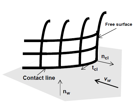
This boundary condition card is used as a distinguishing condition on the mesh motion equations (viz. mesh1, mesh2, and mesh3 under the EQ card). It enforces the boundary of the mesh defined by the side set to conform to a transient or steady material surface, with an optional, pre-specified mass loss/gain rate. This condition is applied only in three-dimensional problems along contact lines that define the intersection of a freesurface and a geometrical solid, the intersection of which is partially characterized by the binormal tangent as described below.

Definitions of the input parameters are as follows:

KINEMATIC_EDGE	Name of the boundary condition (<bc_name>).
SS	Type of boundary condition (<bc_type>), where SS denotes side set in the EXODUS II database.
<bc_id1>	The boundary flag identifier, an integer associated with <bc_type> that identifies the boundary location (side set in EXODUS II) in the problem domain. This surface is the “primary solid surface”
<bc_id2>	The boundary flag identifier, an integer associated with <bc_type> that identifies the boundary location (side set in EXODUS II) in the problem domain. This surface is the “free surface”
<float1>	Mass-loss (positive) or mass-gain (negative) velocity at the free boundary.

Examples#

BC = KINEMATIC_SPECIES SS 10 2 0.0

In this example, the KINEMATIC_EDGE boundary condition is applied to the line defined by the intersection of side sets 10 and 20. The normal vector used in application of this condition is the one in the plane of side-set 10, viz. it is tangent to the surface delineated by side set 10.

Technical Discussion#

The functional form of the kinematic boundary condition is:

\[\underline{n}_{\mathrm{cl}} \cdot \left( \underline{v} - \underline{v}_s \right) = 0\]

Here \(\underline{n}_{\mathrm{cl}}\) is the unit normal tangent vector to a line in space defined by two surfaces, in the plane of the primary surface, viz. tangent to that surface. \(\underline{v}\) is the velocity of the fluid, \(\underline{v}_s\) is the velocity of the surface (or mesh). This condition only makes sense in three dimensions, and needs to be directed with ROT conditions for proper application.

References#

GT-007.2: Tutorial on droplet on incline problem, July 30, 1999, T. A. Baer

KINEMATIC_SPECIES#

BC = KINEMATIC_SPECIES SS <bc_id> <integer>

Description / Usage#

(WIC/MASS)

This boundary condition card is used to impose an interphase species flux continuity constraint on species components undergoing phase change between two materials. The species conservation equation (see EQ card and species_bulk) for a single gas or liquid phase component requires two boundary conditions because of the multivalued, discontinuous concentration at the interface. This condition should be used in conjunction with VL_EQUIL tie condition for each species. Definitions of the input parameters are as follows:

KINEMATIC_SPECIES	Name of the boundary condition (<bc_name>).
SS	Type of boundary condition (<bc_type>), where SS denotes side set in the EXODUS II database.
<bc_id>	The boundary flag identifier, an integer associated with <bc_type> that identifies the boundary location (side set in EXODUS II) in the problem domain.
<integer>	Species number.
<float1>	Unused floating point number.

This boundary condition is typically applied to multicomponent two-phase flows that have rapid mass exchange between phases, rapid enough to induce a diffusion velocity at the interface, and to thermal contact resistance type problems. The best example of this is rapid evaporation of a liquid component into a gas.

Examples#

Following is a sample card:

BC = KINEMATIC_SPECIES SS 10 2 0.0

This card invokes the species flux balance condition on species 2 at shared side set 10 to be applied to the liquid phase convective diffusion equation. It should be used in conjunction with a VL_EQUIL type condition on the same species, but from the bounding phase. Note: side set 10 must be a double-sided side set between two materials (i.e., must be attached to both materials), each deploying basis function interpolation of type Q1_D or Q2_D.

Technical Discussion#

The condition only applies to interphase mass transfer problems with discontinuous (or multivalued) variables at an interface, and it must be invoked on fields that employ the Q1_D or Q2_D interpolation functions to “tie” together or constrain the extra degrees of freedom at the interface in question. The mathematical form is

\[\underline{n} \cdot \left[ \left( \underline{v}_s - {\underline{v}}^l \right) {y_i}^l \rho^l - {\underline{j}_i}^l \right] = \underline{n} \cdot \left[ \left( \underline{v}_s - {\underline{v}}^g \right) {y_i}^g \rho^g - {\underline{j}_i}^g \right]\]

Here \({\underline{v}}^l\) and \({\underline{v}}^g\) are the gas and liquid velocity vectors at the free surface, respectively; \(\underline{v}_s\) is the mesh velocity at the same location; \(\rho^l\) and \(\rho^g\) are the liquid and gas phase densities, respectively; \({y_i}^l\) and \({y_i}^g\) are the liquid and gas phase volume fractions of component \(i\); and \({\underline{j_i}}^l\) and \({\underline{j_i}}^g\) the mass fluxes of component \(i\). This condition constrains only one of two phase concentrations at the discontinuous interface. The other needs to come from a Dirichlet boundary condition like (BC =) Y, or an equilibrium boundary condition like VL_EQUIL.

References#

Schunk, P. R. and Rao, R. R. 1994. “Finite element analysis of multicomponent twophase flows with interphase mass and momentum transport”, Int. J. Numer. Meth. Fluids, 18, 821-842.

GTM-007.1: New Multicomponent Vapor-Liquid Equilibrium Capabilities in GOMA, December 10, 1998, A. C. Sun

KIN_DISPLACEMENT_PETROV#

BC = KIN_DISPLACEMENT_PETROV SS <bc_id> <integer>

Description / Usage#

(SIC/ROTATED MESH)

The KIN_DISPLACEMENT_PETROV boundary condition is exactly the same as KIN_DISPLACEMENT except in the way in which it is applied numerically to a problem. See KIN_DISPLACEMENT for a full discussion.

Definitions of the input parameters are as follows:

KIN_DISPLACEMENT_PETROV	Name of the boundary condition (<bc_name>).
SS	Type of boundary condition (<bc_type>), where SS denotes side set in the EXODUS II database.
<bc_id>	The boundary flag identifier, an integer associated with <bc_type> that identifies the boundary location (side set in EXODUS II) in the problem domain.
<integer>	Element block identification number for the region of TALE solid mesh motion.

Sometimes this condition is a better alternative to KIN_DISPLACEMENT to stabilize the surface and prevent wiggles. If the user wants to know more regarding numerical issues and implementation, consult the description for the fluid-counterpart KINEMATIC_PETROV card.

Examples#

The following sample card:

BC = KIN_DISPLACEMENT_PETROV SS 7 12

leads to the application of the kinematic boundary condition (displacement form, see below) to the boundary-normal component of the mesh-stress equation to the boundary defined by side set 7. The element block ID number which shares this boundary with a neighboring TALE or fluid ARBITRARY region is 12.

Technical Discussion#

See discussions on the KINEMATIC_PETROV and KIN_DISPLACEMENT cards.

References#

No References.

KIN_DISPLACEMENT_COLLOC#

BC = KIN_DISPLACEMENT_COLLOC SS <bc_id> <integer>

Description / Usage#

(SIC/ROTATED MESH)

The KIN_DISPLACEMENT_COLLOC boundary condition is exactly the same as KIN_DISPLACEMENT except in the way in which it is applied numerically to a problem. See KIN_DISPLACEMENT for a full discussion.

Definitions of the input parameters are as follows:

KIN_DISPLACEMENT_COLLOC	Name of the boundary condition (<bc_name>).
SS	Type of boundary condition (<bc_type>), where SS denotes side set in the EXODUS II database.
<bc_id>	The boundary flag identifier, an integer associated with <bc_type> that identifies the boundary location (side set in EXODUS II) in the problem domain.
<integer>	Element block identification number for the region of TALE solid mesh motion.

Examples#

The following sample card:

BC = KIN_DISPLACEMENT_COLLOC SS 7 12

Technical Discussion#

See discussions on the KINEMATIC_COLLOC and KIN_DISPLACEMENT cards.

References#

No References.

KIN_DISPLACEMENT#

BC = KIN_DISPLACEMENT SS <bc_id> <integer>

Description / Usage#

(SIC/ROTATED MESH)

This boundary condition card is used as a distinguishing condition on the mesh motion equations (viz. mesh1, mesh2, and mesh3 under the EQ card). It forces the boundary of the mesh defined by the side set to conform to a transient or steady material surface. Unlike the KINEMATIC condition, which is designed for material surfaces between two fluids, or the external material boundary of a fluid, this condition is applied to solid materials to which the TOTAL_ALE mesh motion scheme is applied (see technical discussion below and the Mesh Motion card). In two dimensions, this condition is automatically applied to the normal component of the vector mesh equations, which is rotated into normal-tangential form. In three dimensions, the application of this boundary condition needs to be further directed with the ROT cards (see ROTATION specifications). The application of this condition should be compared with KIN_DISPLACEMENT_PETROV and KIN_DISPLACEMENT_COLLOC.

Definitions of the input parameters are as follows:

KIN_DISPLACEMENT	Name of the boundary condition (<bc_name>).
SS	Type of boundary condition (<bc_type>), where SS denotes side set in the EXODUS II database.
<bc_id>	The boundary flag identifier, an integer associated with <bc_type> that identifies the boundary location (side set in EXODUS II) in the problem domain.
<integer>	Element block identification number for the region of TALE solid mesh motion.

Examples#

The following sample card:

BC = KIN_DISPLACEMENT SS 7 12

Technical Discussion#

The functional form of the kinematic boundary condition is:

\[\underline n \cdot \left(\underline d_m - \underline d_m^0 \right) - \underline n \cdot \left(\underline d - \underline d^0 \right) = 0\]

Here EQUATION is the unit normal vector to the solid-fluid free surface, EQUATION is the mesh displacement at the boundary EQUATION, is the mesh displacement from the base reference state (which is automatically updated from the stress-free state coordinates and for remeshes, etc. in Goma and need not be specified), EQUATION is the real solid displacement, and EQUATION is the real solid displacement from the base reference state (or mesh). In stark contrast with the KINEMATIC condition, which too is used to distinguish a material fluid surface) this condition is written in Lagrangian displacement variables for TALE mesh motion and is applied as a distinguishing condition on the mesh between a fluid and TALE solid region. In essence, it maintains a real solid displacement field such that no real-solid mass penetrates the boundary described by this condition.

References#

SAND2000-0807: TALE: An Arbitrary Lagrangian-Eulerian Approach to Fluid- Structure Interaction Problems, P. R. Schunk, May 2000

GT-005.3: THE NEW TOTAL-ARBITRARY-LAGRANGIAN-EULERIAN (TALE) CAPABILITY and its applicability to coating with/on deformable media, August 6, 1999, P. R. Schunk

KIN_LEAK#

BC = KIN_LEAK SS <bc_id> <float1> <float2>

Description / Usage#

(SIC/ROTATED MESH)

This boundary condition card is used as a distinguishing condition - kinematic with mass transfer on mesh equations. The flux quantity is specified on a per mass basis so heat and mass transfer coefficients are in units of L/t.

Definitions of the input parameters are as follows:

KIN_LEAK	Name of the boundary condition (<bc_name>).
SS	Type of boundary condition (<bc_type>), where SS denotes side set in the EXODUS II database.
<bc_id>	The boundary flag identifier, an integer associated with <bc_type> that identifies the boundary location (side set in EXODUS II) in the problem domain.
<float1>	Mass transfer coefficient for bulk fluid (species n +1).
<float2>	Driving force concentration in external phase.

Please see Technical Discussion regarding the appropriate units for the mass transfer coefficient and concentration in the external phase. For a pure liquid case, these inputs are read directly from this card, while for a multi-component case these values are read from YFLUX boundary conditions corresponding to each species that is needed. See following examples.

Examples#

Following are two sample input cards:

Pure Liquid Case

BC = KIN_LEAK SS 3   0.1   0.

Two Component Case

BC = KIN_LEAK SS 3   0.   0.

BC = YFLUX SS 3   0   0.12   0.

Note, in the two component case, when Goma finds the KIN_LEAK card, it scans the input deck to locate the applicable YFLUX conditions associated with side set 3 and creates a linked list which is used by the applying function (kin_bc_leak). The existence of this list is denoted in Goma by the addition of an integer into an unused field of the BC structure for side set 3. The bulk fluid constitutes the second component and is non-volatile so it requires no YFLUX card; a second volatile species would require a second YFLUX input card.

Technical Discussion#

Functionally, the KIN_LEAK boundary condition can be represented as the following:

\[\underline n \cdot \left(\underline v - \underline v_s\right) = \sum_{i} h_i \left(y_i - y_i^0\right)\]

where EQUATION is the vector velocity; EQUATION is the velocity of the boundary itself (not independent from the mesh velocity); EQUATION is the normal vector to the surface; EQUATION is the concentration of species i; EQUATION is the ambient concentration of species i at a distance from the surface of interest and EQUATION is the mass transfer coefficient for species i. This function returns a volume flux term to the equation assembly function.

KIN_LEAK is implemented through function kin_bc_leak; it sums the fluxes for all species plus the bulk phase evaporation. These fluxes are computed via several other function calls depending on the particular flux condition imposed on the boundary. (See various YFLUX * cards for Mass Equations.) However, at the end of the kin_bc_leak function, the accumulated flux value is assigned to variable vnormal, i.e., the velocity of fluid relative to the mesh. The apparent absence of a density factor here to convert a volume flux to a mass flux is the crucial element in the proper usage of the flux boundary conditions. The explanation is rooted in the formulation of the convective-diffusion equation.

The convective-diffusion equation in Goma is given as

\[\frac{d y_i}{dt} = - \left(v - v_m\right) \cdot \nabla y_i - \nabla \cdot J_i + R_i\]

with mass being entirely left out of the expression. J is divided by density before adding into the balance equation; this presumes that volume fraction and mass fraction are equivalent. The users must be aware of this. This formulation is certainly inconvenient for problems where volume fraction and mass fraction are not equal and multicomponent molar fluxes are active elements of an analysis. However, kin_bc_leak is entirely consistent with the convective-diffusion equation as a velocity is a volume flux, and multiplied by a density gives a proper mass flux. If y_i is a mass concentration, and h_i were in its typical velocity units, the result is a mass flux; if y_i is a volume fraction, then we have a volume flux. So kin_bc_leak is consistent.

The burden here lies with the user to be consistent with a chosen set of units. A common approach is to build density into the mass transfer coefficient h_i .

FAQs#

See the FAQ pertaining to “Continuation Strategies for Free Surface Flows” on the DISTNG boundary condition card.
A question was raised regarding the use of volume flux in Goma; the following portion of the question and response elucidate this topic and the subject of units. Being from several emails exchanged during January 1998, the deficiencies or lack of clarity have since been remedied prior to Goma 4.0, but the discussions are relevant for each user of the code.

Question: … I know what you are calling volume flux is mass flux divided by density. The point I am trying to make is that the conservation equations in the books I am familiar with talk about mass, energy, momentum, and heat fluxes. Why do you not write your conservation equations in their naturally occurring form? If density just so happens to be common in all of the terms, then it will be obvious to the user that the problem does not depend on density. You get the same answer no matter whether you input rho=1.0 or rho=6.9834, provided of course this does not impact iterative convergence. This way, you write fluxes in terms of gradients with the transport properties (viscosity, thermal conductivity, diffusion coefficient, etc.) being in familiar units.

Answer: … First let me state the only error in the manual that exists with regard to the convection-diffusion equation (CDE) is the following:

J_i in the nomenclature table should be described as a volume flux with units of L/t, i.e., D ⋅ ∇y_i, where D is in L²/t units.

Now, this is actually stated correctly elsewhere, as it states the J_i is a diffusion flux (without being specific); to be more specific here, we should say it is a “volume flux of species i.” So, in this case D is in L ⋅ L/t units y_i, is dimensionless and it is immaterial that the CDE is multiplied by density or not, as long as density is constant.

Now, in Goma we actually code it with no densities anywhere for the FICKIAN diffusion model. For the HYDRO diffusion model, we actually compute a J_i /ρ in the code, and handle variable density changes through that ρ. In that case J_i as computed in Goma is a mass flux vector, not a volume flux vector, but by dividing it by ρ and sending it back up to the CDE it changes back into a volume flux. i. e., everything is the same.

Concerning the units of the mass transfer coefficient on the YFLUX boundary condition, the above discussion now sets those. Goma clearly needs the flux in the following form:

\[\underline n \cdot D \nabla Y = K \cdot \left(p_i - p_i^{\infty}\right)\]

and dimensionally for the left hand side

\[\left(L^2 / t\right) \cdot \left(1/L \right) = L/t\]

where D is in units L²/t, the gradient operator has units of 1/L so K has to be in units of L/t (period!) because y_i is a fraction.

So, if you want a formulation as follows:

\[\underline n \cdot D \nabla Y = K \left(y_i - y_i^{\infty} \right)\]

then K’s units will have to accommodate for the relationship between p_i and y_i in the liquid, hopefully a linear one as in Raoult’s law, i.e. if p_i = PvV_i where Pv is the vapor pressure, then

\[\underline n \cdot D \nabla Y = KP_V \left(y_i - y_i^{\infty} \right)\]

and so K on the YFLUX command has to be KPv….and so on.

Finally, you will note, since we do not multiply through by density, you will have to take care of that, i. e., in the Price paper he gives K in units of t/L. So, that must be converted as follows:

\[ \begin{align}\begin{aligned}K_{price} \left(P_V / p \right) = K_{goma}\\\left(t / L \right) \left(M / L t^2\right) \left(L^3 / M \right) = L/t\end{aligned}\end{align} \]

This checks out!

References#

Price, P. E., Jr., S. Wang, I. H. Romdhane, “Extracting Effective Diffusion Parameters from Drying Experiments,” AIChE Journal, 43, 8, 1925-1934 (1997)

KIN_CHEM#

BC = KIN_CHEM SS <bc_id> <float1> ... <floatn>

Description / Usage#

(SIC/ROTATED MESH)

This boundary condition card is used to establish the sign of flux contributions to the overall mass balance on boundaries so that movements are appropriately advancing or receding depending on whether a species is a reactant or product in a surface reaction.

Definitions of the input parameters are as follows:

KIN_CHEM	Name of the boundary condition (<bc_name>).
SS	Type of boundary condition (<bc_type>), where SS denotes side set.
<bc_id>	The boundary flag identifier, an integer associated with <bc_type> that identifies the boundary location (set in EXODUS II) in the problem domain.
<float1>	Stoichiometric coefficient for species 0.
<floatn>	Stoichiometric coefficient for species n +1.

The input function will read as many stoichiometric coefficients as specified by the user for this card; the number of coefficients read is counted and saved. The stoichiometric coefficient is +1 for products or -1 for reactants. When a species is a product, the surface will advance corresponding to production/creation of mass of that species, versus recession of that interface when a reaction leads to consumption of that species.

Examples#

Following is a sample card for two reactant and one product species:

BC = KIN_CHEM SS 25   -1.0   -1.0   1.0

Technical Discussion#

This function is built from the same function as boundary condition KIN_LEAK, i.e., kin_bc_leak, so the user is referred to discussions for this boundary condition for appropriate details. The stoichiometric coefficients are read from the KIN_CHEM card or set equal to 1.0 in the absence of KIN_CHEM.

References#

No References.

KINEMATIC_XI#

BC = KINEMATIC_XI SS <bc_id> <float1> [integer]

Description / Usage#

(SIC/MESH1)

This is applied on the MESH1 component and is not rotated.

Definitions of the input parameters are as follows:

KINEMATIC_XI	Name of the boundary condition (<bc_name>).
SS	Type of boundary condition (<bc_type>), where SS denotes side set in the EXODUS II database.
<bc_id>	The boundary flag identifier, an integer associated with <bc_type> that identifies the boundary location (side set in EXODUS II) in the problem domain.
<float1>	Mass-loss (positive) or mass-gain (negative) velocity at the free boundary.
[integer]	Optional integer value indicating the element block id from which to apply the boundary condition.

Examples#

The following sample card

BC = KINEMATIC_XI SS 7 0.0

leads to the application of the kinematic boundary condition to the MESH1 component of the mesh equation on the boundary defined by side set 7.

Technical Discussion#

The functional form of the kinematic boundary condition is:

\[\underline{n} \cdot \left( \underline{v} - \underline{v}_s \right) = \dot{m}\]

FAQs#

See the FAQ pertaining to “Continuation Strategies for Free Surface Flows” on the DISTNG boundary condition card.

References#

GT-001.4: GOMA and SEAMS tutorial for new users, February 18, 2002, P. R. Schunk and D. A. Labreche

KINEMATIC_ETA#

BC = KINEMATIC_ETA SS <bc_id> <float1> [integer]

Description / Usage#

(SIC/MESH2)

This is applied on the MESH2 component and is not rotated.

Definitions of the input parameters are as follows:

KINEMATIC_ETA	Name of the boundary condition (<bc_name>).
SS	Type of boundary condition (<bc_type>), where SS denotes side set in the EXODUS II database.
<bc_id>	The boundary flag identifier, an integer associated with <bc_type> that identifies the boundary location (side set in EXODUS II) in the problem domain.
<float1>	Mass-loss (positive) or mass-gain (negative) velocity at the free boundary.
[integer]	Optional integer value indicating the element block id from which to apply the boundary condition.

Examples#

The following sample card

BC = KINEMATIC_ETA SS 7 0.0

leads to the application of the kinematic boundary condition to the MESH1 component of the mesh equation on the boundary defined by side set 7.

Technical Discussion#

The functional form of the kinematic boundary condition is:

\[\underline{n} \cdot \left( \underline{v} - \underline{v}_s \right) = \dot{m}\]

FAQs#

See the FAQ pertaining to “Continuation Strategies for Free Surface Flows” on the DISTNG boundary condition card.

References#

GT-001.4: GOMA and SEAMS tutorial for new users, February 18, 2002, P. R. Schunk and D. A. Labreche

FORCE#

BC = FORCE SS <bc_id> <float1> <float2> <float3>

Description / Usage#

(WIC/VECTOR MESH)

This boundary condition card applies a force per unit area (traction) on a Lagrangian mesh region. The force per unit area is applied uniformly over the boundary delineated by the side set ID. The applied force is of course a vector. Definitions of the input parameters are as follows:

FORCE	Name of the boundary condition (<bc_name>)
SS	Type of boundary condition (<bc_type>), where SS denotes side set in the EXODUS II database.
<bc_id>	The boundary flag identifier, an integer associated with <bc_type> that identifies the boundary location (side set in EXODUS II) in the problem domain.
<float1>	X-component of traction in units of force/area.
<float2>	Y-component of traction in units of force/area.
<float3>	Z-component of traction in units of force/area.

Examples#

Following is a sample card:

BC = FORCE SS 10 0. 1.0 1.0

This card results in a vector traction defined by EQUATION being applied to the side set boundary delineated by the number 10.

Technical Discussion#

Important note: this boundary condition can only be applied to LAGRANGIAN, DYNAMIC_LAGRANGIAN or ARBITRARY mesh motion types (cf. Mesh Motion card). For real-solid mesh motion types, refer to FORCE_RS. Furthermore, it is rare and unlikely that this boundary condition be applied to ARBITRARY mesh motion regions. An example application of this boundary condition card is to address the need to apply some load pressure to a solid Lagrangian region, like a rubber roller, so as to squeeze and drive flow in a liquid region.

FAQs#

On internal two-sided side sets, this boundary condition results in double the force in the same direction.

References#

A MEMS Ejector for Printing Applications, A. Gooray, G. Roller, P. Galambos, K. Zavadil, R. Givler, F. Peter and J. Crowley, Proceedings of the Society of Imaging Science & Technology, Ft. Lauderdale FL, September 2001.

NORM_FORCE#

BC = NORM_FORCE SS <bc_id> <float1> <float2> <float3>

Description / Usage#

(WIC/VECTOR MESH)

This boundary condition card applies a force per unit area (traction) on a Lagrangian mesh region. The force per unit area is applied uniformly over the boundary delineated by the side set ID. The applied traction is of course a vector. Unlike the FORCE boundary condition card, the vector traction here is defined in normal-tangent vector basis. Definitions of the input parameters are as follows:

NORM_FORCE	Name of the boundary condition (<bc_name>).
SS	Type of boundary condition (<bc_type>), where SS denotes side set.
<bc_id>	The boundary flag identifier, or a side set number which is an integer that identifies the boundary location (side set in EXODUS II) in the problem domain.
<float1>	Normal component of traction in units of force/area.
<float2>	Tangential component of traction in units of force/area.
<float3>	Second tangential component of traction in units of force/area (in 3-D).

This card actually applies a traction that is then naturally integrated over the entire side set of elements. Hence, the units on the floating point input must be force/area.

Examples#

Following is a sample card:

BC = NORM_FORCE SS 10   0.   1.0   1.0

This card results in a vector traction defined by EQUATION being applied to the side set boundary delineated by the number 10. The normal vector is defined as the outward pointing normal to the surface. For internal surfaces defined by side sets which include both sides of the interface, this condition will result in exactly a zero traction, i.e., internal surface side sets must be attached to one element block only to get a net effect.

Technical Discussion#

Important note: this boundary condition can only be applied to LAGRANGIAN, DYNAMIC_LAGRANGIAN or ARBITRARY mesh motion types (cf. Mesh Motion card). For real-solid mesh motion types, refer to NORM_FORCE_RS. Furthermore, it is rare and unlikely that this boundary condition be applied to ARBITRARY mesh motion regions. An example application of this boundary condition card is to apply some load pressure uniformly on the inside of a solid-membrane (like a pressurized balloon). In more advanced usage, one could tie this force to an augmenting condition on the pressure, as dictated by the ideal gas law.

This boundary condition is not used as often as the FORCE or FORCE_USER counterparts.

REP_FORCE#

BC = REP_FORCE SS <bc_id> <float_list>

Description / Usage#

(WIC/VECTOR MESH)

This boundary condition card applies a force per unit area (traction) that varies as the inverse of the fourth power of the distance from a planar surface to a Lagrangian or dynamic Lagrangian mesh region. This boundary condition can be used to impose a normal contact condition (repulsion) or attraction condition (negative force) between a planar surface and the surface of a Lagrangian region. The force per unit area is applied uniformly over the boundary delineated by the side set ID. The applied force is a vector in the normal direction to the Lagrangian interface.

Definitions of the input parameters are as follows, with <float_list> having five parameters:

REP_FORCE	Name of the boundary condition (<bc_name>)
SS	Type of boundary condition (<bc_type>), where SS denotes side set in the EXODUS II database.
<bc_id>	The boundary flag identifier, an integer associated with <bc_type> that identifies the boundary location (side set in EXODUS II) in the problem domain.
<float1>	Coefficient of repulsion, λ.
<float2>	Coefficient a of plane equation.
<float3>	Coefficient b of plane equation.
<float4>	Coefficient c of plane equation.
<float5>	Coefficient d of plane equation.

Refer to the Technical Discussion for an explanation of the various coefficients.

Examples#

The following sample card:

BC = FORCE_REP SS   10  1.e+03.   1.0   0.0 0.0   -3.0

results in a vector traction of magnitude –1.0e3 ⁄ h⁴ in the normal direction to surface side set 10 and the distance h is measured from side set 10 to the plane defined by 1.0x – 3. = 0.

Technical Discussion#

The REP_FORCE boundary condition produces a vector traction in the normal direction to a surface side set, defined by:

\[\vec{F} = F (\vec{n}) = - \frac{\lambda}{h^4}\]

where F is a force per unit area that varies with the distance h from a plane defined by

\[ax + by + cz + d = 0\]

The normal vector is defined as the outward pointing normal to the surface. For internal surfaces defined by side sets which include both sides of the interface, this condition will result in exactly a zero traction, i.e., internal surface side sets must be attached to one element block only to get a net effect.

Important note: this boundary condition can only be applied to LAGRANGIAN, DYNAMIC_LAGRANGIAN or ARBITRARY mesh motion types (cf. Mesh Motion card). For real-solid mesh motion types, refer to REP_FORCE_RS. Furthermore, it is rare and unlikely that this boundary condition be applied to ARBITRARY mesh motion regions. An example application of this boundary condition card is to apply some load pressure uniformly on a surface that is large enough such that this surface never penetrates a predefined planar boundary. Hence, this condition can be use to impose an impenetrable contact condition.

FAQs#

On internal two-sided side sets, this boundary condition results in double the force in the same direction.

FORCE_USER#

BC = FORCE_USER SS <bc_id> <float1> ...<floatn>

Description / Usage#

(WIC/VECTOR MESH)

This boundary condition card applies a user-defined force per unit area (traction) on a Lagrangian or dynamic Lagrangian (see Mesh Motion card) mesh region. The functional form of the force is programmed in the function force_user_surf in bc_user.c, and can be made a function of any of the independent or dependent variables of the problem, including position (see example below). The force per unit area is applied to boundary delineated by the side set ID. Definitions of the input parameters are as follows:

FORCE_USR	Name of the boundary condition (<bc_name>)
SS	Type of boundary condition (<bc_type>), where SS denotes side set in the EXODUS II database.
<bc_id>	The boundary flag identifier, an integer associated with <bc_type> that identifies the boundary location (side set in EXODUS II) in the problem domain.
<float1>…<floatn>	Parameters list (length arbitrary) for parameterizing the user defined force. These parameters are accessed through the p[]array in force_user_surf.

Examples#

The input card

BC = FORCE_USER SS 3   {delta_t} 0.   1000.0 0.

used in conjuction with the following snippet of code in force_user_surf:

/* Comment this out FIRST!!!!! */
   /* EH(-1,"No FORCE_USER model implemented"); */
   /**************************** EXECUTION BEGINS
   *******************************/
   if (time <= p[0])
   {
           func[0] = p[1]*time/p[0];
           func[1] = p[2]*time/p[0];
           func[2] = p[3]*time/p[0];
   }
   else
   {
           func[0] = p[1];
           func[1] = p[2];
           func[2] = p[3];
   }

applies a time-dependent force ramped from zero to 1000.0 in the +y direction over the time period {delta_t}.

Technical Discussion#

Used commonly to apply a force per unit area to an external surface of a solid region (LAGRANGIAN type, cf. FORCE_USER_RS), that is nonconstant, viz. time varying or spatially varying. The FORCE and NORM_FORCE boundary conditions can be used for constant forces. This condition is applied as a weak integrated condition in Goma, and hence will be additive with others of its kind.

FAQs#

On internal two-sided side sets, this boundary condition results in double the force in the same direction.

References#

No References.

CA#

BC = CA NS <bc_id> <float_list>

Description / Usage#

(PCC/ROTATED MESH)

This boundary condition card applies a specified contact-angle on the mesh at a single node nodeset. It is used exclusively in two dimensional computations. Its primary application is imposing contact angles at static or dynamic contact lines. Consequently, the nodeset is usually found where a free-surface boundary intersects a fixed, “geometry” boundary.

The <float_list> for this boundary condition has four values; definitions of the input parameters are as follows:

CA	Name of the boundary condition.
NS	Type of boundary condition (<bc_type>), where NS denotes node set in the EXODUS II database.
<bc_id>	The boundary flag identifier, an integer associated with <bc_type> that identifies the boundary location (node set in EXODUS II) in the problem domain.
<float1>	θ, angle subtended by wall normal and free surface normal, in units of radians.
<float2>	n_x, x-component of normal vector to the geometry boundary (see important note below regarding variable wall normals, viz. non-planar solid walls).
<float3>	n_y, y-component of normal vector to the geometry boundary. (see important note below regarding variable wall normals, viz. non-planar solid walls).
<float4>	n_z, z-component of normal vector to the geometry boundary. (see important note below regarding variable wall normals, viz. non-planar solid walls).

Examples#

Following is a sample card:

BC = CA NS 100 1.4 0. 1. 0.

This condition applies a contact angle of 1.4 radians between the free surface normal at the 100 nodeset and the vector (0,1,0). Normally, this latter vector is the normal to the solid surface in contact with the free surface at this point.

Technical Discussion#

The constraint that is imposed at the nodeset node is:

\[\underline n \cdot \underline n_{fs} = cos \ \theta\]

where n is the normal to the geometry specified on the card itself, and n_fs is the normal to the outward free surface computed internally by Goma. Also see the CA_OR_FIX card for an extension to this condition and CA_EDGE for its extension to three dimensions.
In addition for the case in which the geometry normal components are set to zero, the wall normal is allowed to vary with a geometrical boundary condition, i.e., GD_TABLE, SPLINE, PLANE, etc. The geometry normal is found on the same or on a neighboring element that contains the dynamic contact angle in question. If a GD*_ type boundary condition is used to describe the wall (i.e., *GD_TABLE), one must specify the R_MESH_NORMAL equation type on that equation for the variable wall normal to take effect.
Important: Variable Wall Normals. Situations for which the wall shape is nonplanar, meaning that the normal vector is not invariant as the contact line moves, there is an option to leave all of the normal-vector components zero. In this case Goma then seeks to determine the local wall normal vector from the geometry it is currently on, using the element facets. It is recommended that this option not be used unless the geometry is truly nonplanar, as the logic is complex and not 100% reliable. An example of such a case is as follows:

BC = CA NS 100 1.4 0. 0. 0.

Notice how all three components of the normal vector are set to zero.

Important: Wall Normal convention. The wall normal vector on an external solid boundary is defined in goma as the inward facing normal to the mesh, and the free surface normal to the liquid (or wetting phase for two-liquid systems) is defined as the outward facing normal to the free surface. Put another way and referring to the picture below, the wall normal is directed from the “solid phase” to the “liquid phase”, and the free surface normal is directed from the “liquid phase” or “wetting phase” to the “vapor phase” or “Non-wetting phase”. Note that for zero contact angle the liquid is “perfectly wetting”. The air-entrainment limit (viz. the hydrodynamic theory interpretation) would occure at a 180 degree contact angle. Recall that the angle is specified in radians on this card.

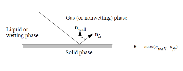
References#

No References.

CA_OR_FIX#

BC = CA_OR_FIX NS <bc_id> <float_list>

Description / Usage#

(PCC/ROTATED MESH)

This boundary condition card allows the application of Gibb’s inequality condition in conjuction with a contact angle. This allows for a point to be specified at which a contact line will attach itself and no longer move. Up to that point, the contact line will advance or recede with a specified fixed contact angle. When the contact line attaches, its contact angle is allowed to vary permitting the user to include discontinuities in surface slope as features of the problem. The Gibb’s condition also permits the contact line to detach from its fixed point if the contact angle enters a certain range after attaching. This boundary condition is applicable only to two-dimensional problems; see CA_EDGE_OR_FIX for details on three dimensional implementations.

The <float_list> has seven values, with definition of the input parameters as follows:

CA_OR_FIX	Name of the boundary condition.
NS	Type of boundary condition (<bc_type>), where NS denotes node set in the EXODUS II database.
<bc_id>	The boundary flag identifier, an integer associated with <bc_type> that identifies the boundary location (node set in EXODUS II) in the problem domain.
<float1>	θ_dcl, dynamic contact angle, in radians.
<float2>	n_x, x-component of outward-pointing wall surface normal.
<float3>	n_y, y-component of outward-pointing wall surface normal.
<float4>	n_z, z-component of outward-pointing wall surface normal.
<float5>	x₀, x-coordinate of the point or feature at which the meniscus will pin.
<float6>	y₀, y-coordinate of the point or feature at which the meniscus will pin.
<float7>	z₀, z-coordinate of the point or feature at which the meniscus will pin.

Examples#

Following is a sample card:

BC = CA_OR_FIX NS 100 1.3 0. 1. 0. -0.5 1. 0.

Technical Discussion#

The Gibb’s inequality condition is illustrated in the accompanying figure. The fixed point is indicated by the plane, x = x₀. Initially, the contact line is far from this point as the condition at the contact line fixes the contact angle to the value θ_dcl. However, when the contact line approaches to within ε (1.e-6) of the fixed point, it attaches there and stops moving. The contact angle condition is no longer enforced and the angle of the free surface with respect to the solid normal vector is allowed to vary freely. The other part of the Gibb’s inequality is illustrated (above) by the last sketch. Here, by virture of the overall fluid mechanics, the contact angle withdraws until it is larger than θ_dcl. When this happens the contact line is no longer affixed at x = x₀ and is allowed to move freely. Once again the contact angle condition is enforced.

../../_images/056_goma_physics.png — Contact angles and Gibb’s inequality condition in Goma, for the special case when the meniscus is moving along a surface of constant x.#

Also, please see the important note under the BC = CA card regarding the convention used for specifying wall and free surface normal vectors.

Theory#

The principle behind this condition applies when a contact line encounters a sharp feature on a surface. The feature from a distance might appear as a sharp corner at which the meniscus/contact line prefers to locate rather than undergo continued migration. Actually on a smaller scale, the corner feature is not infinitely small, and the contact line undergoes no perceptable movement on the macroscale in order to satisfy a true contact angle. Rather than resolving this feature with a fine mesh, it is an expedient to pin the contact line there and allow it to take on any macroscale contact angle within a certain range. The line can release again if the meniscus pulls the contact line sufficiently to overcome specified bounds.

References#

No References.

CA_EDGE#

BC = CA_EDGE SS <bc_id1> <bc_id2> <float_list>

Description / Usage#

Warning

The angle in this BC is specified in degrees, not radians. This is different than the 2D equivalent.

(PCC-EDGE/ROTATED MESH)

This boundary condition card specifies a constant contact angle on the edge defined by the intersection of the primary and secondary side sets. This card is used most often to enforce contact angle conditions on three-dimensional static contact lines. It should not be used in two-dimensional problems, where the CA boundary condition is the appropriate choice.

The contact angle supplied on the card will be enforced so that it is the angle between the outward-pointing normal of the primary side set and the unit vector supplied on the card. It is important to note that this outward-pointing normal should be variable, that is to say, the primary side set is most likely a free-surface.

Definitions of the input parameters are as follows:

CA_EDGE	Name of the boundary condition.
SS	Type of boundary condition (<bc_type>), where SS denotes side set in the EXODUS II database.
<bc_id1>	The boundary flag identifier, an integer associated with <bc_type> that identifies the boundary location (side set in EXODUS II) in the problem domain. This identifies the primary side set; in almost all cases it should also be a free surface.
<bc_id2>	The boundary flag identifier, an integer associated with <bc_type> that identifies the boundary location (side set in EXODUS II) in the problem domain. This identifies the secondary side set, which plays no other role in this boundary condition than to provide a means of defining the appropriate edge geometry in conjunction with the primary side set. Thus, the secondary side set will often represent a solid boundary.
<float1>	angle, value specifying the enforced angle, in degrees; it should lie in the range 0 ≤ angle ≤ 180.
<float2>	n_x, the x-component of the fixed unit vector.
<float3>	n_y, the y-component of the fixed unit vector.
<float4>	n_z, the z-component of the fixed unit vector.

This boundary condition is a point collocated condition so it will be enforced exactly at every node that lies on the edge (subject to overriding ROT cards or Dirichlet conditions).

Examples#

The following is a sample input card:

BC = CA_EDGE SS 40 50 33.0 0. 1. 0.

This card will result in an angle of 33 degrees between the outward-pointing normal to side set 40 and the vector (0,1,0) at all points on the edge defined by the intersection of side set 40 and side set 50.

Technical Discussion#

Although this constraint deals with vector quantities, it is a scalar constraint. The actual requirement that is imposed is:

\[n_f \cdot n = cos\ \left(\theta \right)\]

where n_f is the outward-pointing normal to the primary side set, n is the vector supplied on the card, and θ is the angle supplied on the card. It should be recognized that there are usually two orientations for n_f which would satisfy this constraint. Most often the surrounding physics will choose the correct one, but there is nothing to guarantee this in special situations, for example, values for θ near zero or near 180.
This boundary condition is a point collocated condition so the preceding constraint, will be enforce exactly and strongly for each node on the edge. The actual free surface normal is an average of vectors supplied by adjacent elements sharing a given node.
As noted above, this boundary condition is most often used in three-dimensional free surface problems to enforce static contact angle conditions at the junction of a free, capillary surface and a solid boundary. The normal vector supplied on the card would be the normal to this solid boundary. Since this vector is a constant, there is the restriction that in this application this boundary condition can only be used to specify a contact angle with respect to a planar solid boundary. A different boundary condition, CA_EDGE_CURVE, should be used if the solid boundary is not planar.
Related boundary conditions: CA_EDGE_INT, CA_EDGE_CURVE, CA_EDGE_CURVE_INT, VAR_CA_EDGE, VAR_CA_USER.

References#

No References.

CA_EDGE_INT#

BC = CA_EDGE_INT SS <bc_id1> <bc_id2> <float_list>

Description / Usage#

Warning

The angle in this BC is specified in degrees, not radians. This is different than the 2D equivalent.

(SIC-EDGE/ROTATED MESH)

This boundary condition card specifies a constant contact angle on the edge defined by the intersection of the primary and secondary side sets. It is identical in format and function as the CA_EDGE boundary condition. The only difference is that this boundary condition is a strong integrated constraint.

Definitions of the input parameters are as follows:

CA_EDGE_INT	Name of the boundary condition.
SS	Type of boundary condition (<bc_type>), where SS denotes side set in the EXODUS II database.
<bc_id1>	The boundary flag identifier, an integer associated with <bc_type> that identifies the boundary location (side set in EXODUS II) in the problem domain. This identifies the primary side set; in almost all cases it should also be a free surface.
<bc_id2>	The boundary flag identifier, an integer associated with <bc_type> that identifies the boundary location (side set in EXODUS II) in the problem domain. This identifies the secondary side set, which plays no other role in this boundary condition than to provide a means of defining the appropriate edge geometry in conjunction with the primary side set. Thus, the secondary side set will often represent a solid boundary.
<float1>	angle, value specifying the enforced angle, in degrees; it should lie in the range 0 ≤ angle ≤ 180.
<float2>	n_x, the x-component of the fixed unit vector.
<float3>	n_y, the y-component of the fixed unit vector.
<float4>	n_z, the z-component of the fixed unit vector.

Examples#

The following is a sample input card:

BC = CA_EDGE_INT SS 40 50 33.0 0. 1. 0.

Technical Discussion#

As noted above, this boundary condition is identical in function to the CA_EDGE condition. It differs only in the manner of its application. Whereas, the former was a point collocated constraint, this boundary condition strongly enforces the following integrated constraint at a node i**:

\[\int_{\Gamma} \phi_i \left(n_f \cdot n - cos\ (\theta) \right) d \Gamma = 0\]

where φ_i is the finite element trial function for node i, Γ is the edge space curve, n:sub: f is the outward-pointing normal to the primary sideset, n is the vector supplied on the card, and θ is the angle supplied on the card. Because it is an integrated constraint, evaluation of the free-surface normal vector is done at integration points between nodes on the edge. Therefore, there is no averaging of normal vectors. This is sometimes advantageous when there are discontinuities in the slope of the edge curve.

Related boundary conditions: CA_EDGE, CA_EDGE_CURVE, CA_EDGE_CURVE_INT, VAR_CA_EDGE, VAR_CA_USER.

References#

No References.

CA_EDGE_OR_FIX#

BC = CA_EDGE_OR_FIX SS <bc_id1> <bc_id2> <type_string> {float_list}

Description / Usage#

(PCC/ROTATED MESH)

In analogy to the two-dimensional condition, CA_OR_FIX, boundary condition, this boundary condition imposes a contact angle on an edge feature in a three-dimensional mesh. However, this condition also permits the user to specify a closed curve on the substrate plane on which the contact line will attach and not move past. This permits modeling of geometric features in which the substrate slope is discontinuous. When contact lines encounter such sharp features, usually they arrest. The boundary condition also permits the contact line to release from the curve if the overall fluid mechanics would promote a recession of the contact line.

Description of the card parameters is as follows:

CA_EDGE_OR_FIX	Name of boundary condition.
SS	Type of boundary condition (<bc_type>), where SS denotes side set in the EXODUS II database.
<bc_id1>	The boundary flag identifier, an integer associated with <bc_type> that identifies the boundary location (side set in EXODUS II) in the problem domain. This identifies the primary side set defining the edge curve on which this condition applies.
<bc_id2>	The boundary flag identifier, an integer associated with <bc_type> that identifies the boundary location (side set in EXODUS II) in the problem domain. This identifies the secondary side set defining the edge curve on which this condition applies. Taken together, the edge curve is the intersection of the primary and secondary sidesets.
<type_string>	A string identifying the type of feature curve being defined; currently, there are only two choices: CIRCLE and USER. The CIRCLE options indicates that the surface feature on which a Gibb’s criterion is applied is a circle in the substrate plane. The USER option indicates that the user will have to provide a geometric definition in the user subroutine user_gibbs_criterion in the file user_bc.c.
{float_list}	A list of float parameters to be used in defining the contact angle, the normal to the substrate, and other geometric parameters used to define the feature curve. For each <type_string> choice there is a different set of float parameters:
	CIRCLE <float_list>
	<float1>	θ_dcl, contact angle at dynamic contact line, in radians
	<float2>	n_x, x-component of outward substrate normal
	<float3>	n_y, y-component of outward substrate normal
	<float4>	n_z, z-component of outward substrate normal
	<float5>	c_x, x coordinate of circle center
	<float6>	c_y, y-coordinate of circle center
	<float7>	c_z, z-coordinate of circle center
	<float8>	r, radius of circle
	The sign of this last parameter is important. If negative, the implication is that the starting location of the contact line is outside of the circle. If positive, the original location is assumed to be completely inside the circle.
	USER <float_list>
	<floati>	a list of float values that are passed to the function user_gibbs_criterion in the one-dimensional array p in the order in which they appear on the card from left to right. The user must be certain that the parameters appearing here are sufficient for applying the Gibbs criterion as well as imposing the appropriate contact angle.

Examples#

An example making use of the CIRCLE feature curve option is as follows:

BC = CA_EDGE_OR_FIX SS 10 20 CIRCLE 1.3   0. -1. 0.   0. 0. 0.   1.0

This card applies to the intersection between side sets 10 and 20. The constant contact angle applied is 1.3 radians. The substrate outward normal is (0, -1, 0). The feature is a circle of radius 1.0 centered at (0.0, 0.0, 0.0). The original location for the contact line must be completely inside of the feature circle. Note also that the circle center should lie in the substrate plane.

Technical Discussion#

See the Technical Discussion under the boundary condition CA_OR_FIX for a detailed discussion of the nature of the Gibb’s criterion as it applies to contact lines. In a nutshell, however, the basic notion is that the contact line is free to advance over the substrate with an imposed contact angle, constant or dependent on the local conditions. When the contact angle encounters the geometric feature defined in the function user_gibbs_criterion, it is captured at that point and no longer advances. The contact angle is allowed to vary as long as it is held at the feature. The boundary condition also permits the contact line to release from the feature curve and recede the way it came if the contact angle ever becomes larger than its mobile value.
So the phenomena that can be modeled with this boundary condition are those in which a contact line moves to, for example, the edge of cylinder. At the edge, the very small curvature of this feature effectively presents a barrier to further advance of the contact line provided the deformation of the free surface beyond the vertical boundaries of the cylinder is not too large. In the fullness of time, it might also be the case that the free surface is drawn backwards in the direction of the cylinder axis. The contact line should also recede and this boundary condition permits this once the contact angle it makes with the cylinder top exceeds the mobile contact angle by a small amount.

References#

No References.

CA_EDGE_CURVE#

BC = CA_EDGE_CURVE SS <bc_id1> <bc_id2> <float1>

Description / Usage#

(PCC-EDGE/ROTATED MESH)

This boundary condition allows the user to specify a constant contact angle along an edge in three-dimensions. It is similar in function to the CA_EDGE boundary condition in which the contact angle is enforced with respect to a fixed vector. However, for this boundary condition, the contact angle is enforced with respect to the normal of the secondary side set thereby permitting a contact angle constraint to be applied on a curving surface. The boundary condition is applied to the edge curve defined by the intersection of the primary and secondary side sets.

Definitions of the input parameters are as follows:

CA_EDGE_CURVE	Name of the boundary condition.
SS	Type of boundary condition (<bc_type>), where SS denotes side set in the EXODUS II database.
<bc_id1>	The boundary flag identifier, an integer associated with <bc_type> that identifies the boundary location (side set in EXODUS II) in the problem domain. This identifies the primary side set; in almost all cases it should also be a free surface.
<bc_id2>	The boundary flag identifier, an integer associated with <bc_type> that identifies the boundary location (side set in EXODUS II) in the problem domain. This identifies the secondary side set. The outwards-pointing normal vector to this side set is used as the substrate vector when enforcing the contact angle constraint.
<float1>	the enforced contact angle, in degrees. Its value should lie in the range 0 ≤ angle ≤ 180.

Examples#

The following is a sample input card:

BC = CA_EDGE_CURVE SS 40 50 135.0

This boundary condition will enforce a 135 degree angle between the normal to the free surface on side set 40 and the outward-pointing normal to side set 50 at all points along the edge defined by side set 40 and 50. There is no restriction on whether side set 50’s normal vectors must be constant.

Technical Discussion#

Although this boundary condition deals with vector quantities it is a scalar constraint. The actual requirement that is imposed is:

\[n_f \cdot n_s = cos\ \left(\theta \right)\]

where n_f is the outward-pointing normal to the primary side set, n_s is the outward-pointing normal to the secondary side set, and θ is the angle supplied on the card. There is always some confusion regarding the sense of the angle; use the figure to the right for guidance. Note that the sense depicted here is at odds with the usual contact angle convention. Keep this in mind when using this card.
As in the case of the CA_EDGE condition, this condition is also a strongly enforced point collocated condition.
Related boundary conditions: CA_EDGE, CA_EDGE_INT, CA_EDGE_CURVE_INT, VAR_CA_EDGE, VAR_CA_USER.

References#

No References.

CA_EDGE_CURVE_INT#

BC = CA_EDGE_CURVE_INT SS <bc_id1> <bc_id2> <float1>

Description / Usage#

(SIC/ROTATED MESH)

This boundary condition allows the user to specify a constant contact angle along an edge in three-dimensions. It is identical in function to CA_EDGE_CURVE boundary condition, but applies as a strongly integrated constraint. The boundary condition is applied to the edge curve defined by the intersection of the primary and secondary side sets.

Definitions of the input parameters are as follows:

CA_EDGE_CURVE_INT	Name of the boundary condition.
SS	Type of boundary condition (<bc_type>), where SS denotes side set in the EXODUS II database.
<bc_id1>	The boundary flag identifier, an integer associated with <bc_type> that identifies the boundary location (side set in EXODUS II) in the problem domain. This identifies the primary side set; in almost all cases it should also be a free-surface.
<bc_id2>	The boundary flag identifier, an integer associated with <bc_type> that identifies the boundary location (side set in EXODUS II) in the problem domain. This identifies the secondary side set. The outwards-pointing normal vector to this side set is used as the substrate vector when enforcing the contact angle constraint.
<float1>	the enforced contact angle, in degrees. Its value should lie in the range 0 ≤ angle ≤ 180.

Examples#

The following is a sample input card:

BC = CA_EDGE_CURVE_INT SS 40 50 135.0

This boundary condition will enforce a 135 degree angle between the normal to the free surface on side set 40 and the outward-pointing normal to side set 50 at all points along the edge defined by side set 40 and 50. The is no restriction on whether side set 50’s normal vectors must be constant.

Technical Discussion#

Although this boundary condition deals with vector quantities it is a scalar constraint. As noted above the form of the constraint is identical to that in the CA_EDGE_CURVE boundary. In this case, it is applied as a strong integrated constraint:

\[\int_{\Gamma} \phi_i \left(n_f \cdot n_s - cos\ (\theta) \right) d \Gamma = 0\]

where φ_i is the finite element trial function for node i, Γ is the edge space curve, n_f is the outwardpointing normal to the primary sideset, n_s is the outward-pointing normal to the secondary sideset, and θ is the angle supplied on the card. There is always some confusion regarding the sense of the angle. Use the figure to the right for guidance. Note that the sense depicted here is at odds with the usual contact angle convention. Keep this in mind when using this card.
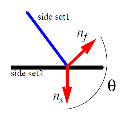
As in the case of the CA_EDGE_INT condition, this condition is also a strongly integrated constraint.
Related boundary conditions: CA_EDGE, CA_EDGE_INT, CA_EDGE_CURVE, VAR_CA_EDGE, VAR_CA_USER.

References#

No References.

VAR_CA_EDGE#

BC = VAR_ CA_EDGE SS <bc_id1> <bc_id2> <float_list>

Description / Usage#

Warning

The angle in this BC is specified in degrees, not radians. This is different than the 2D equivalent.

(SIC-EDGE/ROTATED MESH)

This card is used to set a variable contact angle on a dynamic three-dimensional contact line. A local contact angle is determined based upon the local rate of advance/recession of the contact line with respect to a web, and is always associated with the secondary sideset. This card specifies the static contact angle, θ_s, and a linear proportionality constant c_T between the local advance/recession rate and the cosine of the contact angle. The speed of the moving web is specified by components of the web velocity. The contact angle is imposed between the outward-pointing normal of the primary sideset and the outward-pointing normal of the secondary sideset.

Definitions of the input parameters are as follows:

VAR_CA_EDGE	Name of the boundary condition.
SS	Type of boundary condition (<bc_type>), where SS denotes side set in the EXODUS II database.
<bc_id1>	The boundary flag identifier, an integer associated with <bc_type> that identifies the boundary location (side set in EXODUS II) in the problem domain. This identifies the primary side set; it should be a free surface.
<bc_id2>	The boundary flag identifier, an integer associated with <bc_type> that identifies the boundary location (side set in EXODUS II) in the problem domain. This identifies the secondary side set, which should be a “fixed” geometric entity, e.g. PLANE or SPLINE. Taken together, the primary and secondary sidesets define an edge over which this boundary is applicable.
<float1>	θ_s, parameter that is the static contact angle, in degrees. This is the contact angle that the fluid approaches when the relative motion of the contact line and substrate is zero.
<float2>	c_T, parameter that is the linear proportionality constant between the local advance/recession rate and the cosine of the contact angle; see details below in the Technical Discussion.
<float3>	W_x, x-component of the substrate velocity.
<float4>	W_y, y-component of the substrate velocity.
<float5>	W_z, z-component of the substrate velocity.

Examples#

The following is a sample input card:

BC = VAR_CA_EDGE SS 60 20   135. 0.02   0. -1. 0.

This card sets a variable contact angle condition on the edge between side sets 60 and 20. The static contact angle is 135 degrees and the slope parameter is 0.02. The solid substrate is moving at the fixed velocity (0, -1., 0.).

Technical Discussion#

A contact line that moves relative to its underlying solid substrate is referred to as a dynamic contact line. For a dynamic contact line associated with threedimensional flows, it is recognized that the dynamic contact angle must change from point to point along the curve because the local advance/recession rate of the contact line with respect to the substrate changes. Taking this variability into account is the function of this card.

To understand the function of this card, we first define that the advance (or recession) rate of the contact line, u_wet, as the normal component of the contact line velocity, x_cl , relative to the substrate velocity, W:

\[u_{wet} = n_{cl} \cdot \left(W - \dot x_{cl} \right)\]

where n_cl is a unit vector normal to the contact line in the plane of the substrate as illustrated in the sketch at right. For an advancing contact line u_wet is negative and the converse. We can also define a local capillary number by nondimensionalizing the advance rate as follows,

\[Ca_L = \mu u_{wet} / \sigma\]

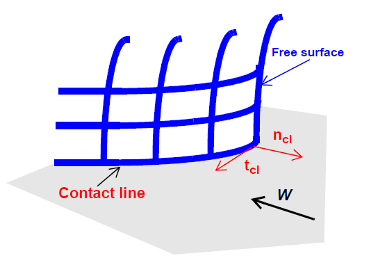
where μ is the viscosity and σ the surface tension.

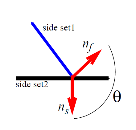
We choose to define the contact angle as the angle between the outward normal to the free-surface and the substrate normal pointing away from the fluid phase as illustrate here. From direct observation of contact lines, we know that increasing the advance rate will decrease the contact angle towards zero. Conversely, a decrease in the advance rate or increase of recession rate will increase the contact angle towards 180. We capture the essence of this behavior via a simple linear relationship between the local capillary number and the cosine of the contact angle:

\[cos\ \theta = cos\ \theta_s - c_T Ca_L\]

where θ_s and c_T are two input parameters. The function of this card is to apply this model for contact angle on the contact line curve.

This model has many restrictions. It is really only valid for very very small | Ca_L | and also does not predict that the contact angle asymptotically approaches 0 or 180 for | Ca_L | very large. Instead, it is algorithmically restricted to returning 0 or 180 if the above linear relation would predict an angle outside of these bounds.
Unlike the CA_EDGE boundary condition, the VAR_CA_EDGE condition is applied as a strong integrated constraint. The equation associated with each node on the edge is:

\[\int_{\Gamma} \phi_i \left(n_f \cdot n_s - (cos\ \theta_s - c_T Ca_L)\right) d \Gamma = 0\]

where φ_i is the shape function associated with node i.

References#

No References.

VAR_CA_USER#

BC = VAR_CA_USER SS <bc_id1> <bc_id2> <float_list>

Description / Usage#

(SIC-EDGE/ROTATED MESH)

This card is used to set a variable contact angle on a dynamic three-dimensional contact line. It is identical in function to the VAR_CA_USER except that it allows the user to provide a contact angle model to relate local contact angle to local capillary number.

Definitions of the input parameters are as follows:

VAR_CA_USER	Name of the boundary condition.
SS	Type of boundary condition (<bc_type>), where SS denotes side set in the EXODUS II database.
<bc_id1>	The boundary flag identifier, an integer associated with <bc_type> that identifies the boundary location (side set in EXODUS II) in the problem domain. This identifies the primary side set; it should be a free surface.
<bc_id2>	The boundary flag identifier, an integer associated with <bc_type> that identifies the boundary location (side set in EXODUS II) in the problem domain. This identifies the secondary side set, which should be a “fixed” geometric entity, e.g. PLANE or SPLINE. Taken together, the primary and secondary sidesets define an edge over which this boundary is applicable.
<float1>	W_x, x-component of the substrate velocity.
<float2>	W_y, y-component of the substrate velocity.
<float3>	W_z, z-component of the substrate velocity.
[float4-floatn]	An optional list of floats which will be passed to the user-supplied function for use with the user model.

Examples#

The following is a sample input card:

BC = VAR_CA_USER SS 60 20   -1. 0. 0. 1.e-3 135.0

This card sets a variable contact angle condition on the edge between side sets 60 and 20. The solid substrate is moving at the fixed velocity (-1., 0., 0.). The var_CA_user function is passed the constants 1.e-3 and 135.0 in variable locations p[0] and p[1], respectively.

Technical Discussion#

VAR_CA_USER function is identical to VAR_CA_EDGE. It is applied to threedimensional dynamic contact lines in order to set a variable contact angle. The user must supply internal coding for the function var_CA_user in the file user*_bc.c. This function receives as parameters the local capillary number as described under *VAR_CA_EDGE and a double array containing the optional list of float parameters. It should return the cosine of the desired contact angle.
What follows is an example that implements the linear contact angle model described in VAR_CA_EDGE.

 double
 var_CA_user(double Ca_local,
            int num,
            const double *a,
            double *d_cos_CA_Ca_local)
{
 double cos_CA;
 double static_CA;
 double cT;
 static_CA = a[0]*M_PIE/180.0;
 cT = a[1];
 cos_CA = cos(static_CA) - cT * Ca_local;
 *d_cos_CA_Ca_local = cT;
 return ( cos_CA );
}

References#

No References.

FRICTION#

BC = FRICTION SS <bc_id> <float1> [integer1]>

Description / Usage#

(WIC/VECTOR MESH)

This boundary condition card applies a force per unit area (traction) on a Lagrangian mesh region. The force per unit area is applied according to Coulomb’s friction law over the boundary delineated by the side set ID. The applied traction is of course a vector. The vector traction is defined in normal-tangent vector basis. Definitions of the input parameters are as follows:

FRICTION	Name of the boundary condition (<bc_name>).
SS	Type of boundary condition (<bc_type>), where SS denotes side set.
<bc_id>	The boundary flag identifier, or a side set number which is an integer that identifies the boundary location (side set in EXODUS II) in the problem domain.
<float1>	\(\mu\), Coulombic coefficient of friction.
[integer1]	optional specification of the element block id to which this condition will be applied.

This card actually applies a traction that is then naturally integrated over the entire side set of elements.

Examples#

Following is a sample card:

BC = FRICTION SS 10 0.1 2

Technical Discussion#

This condition should be utilized in conjunction with a rotated condition such as SPLINE in order to apply a tangential force which is proportional to the normal force;

\[\underline F = \mu F_n \frac{\underline v}{|\underline v|}\]

where \(\mu\) is the coefficient of friction and \(\underline{v}\) is the velocity of the convected solid. Note that the direction of the frictional force is determined by the velocity direction.

SOLID_FLUID#

BC = SOLID_FLUID SS <bc_id> <integer1> <integer2> [float]

Description / Usage#

(PCC/VECTOR REALSOLID)

The SOLID_FLUID condition performs the exact same task as the FLUID_SOLID condition. The usage and example are also the same, so consult the discussion on that card for further information.

At one time this condition applied the stress balance between solid and fluid phases in a different fashion that proved not to be useful. To preserve backward compatibility, we have kept this boundary condition around even though it invokes the exact same function that the FLUID_SOLID boundary condition does.

Definitions of the input parameters are as follows:

SOLID_FLUID	Name of the boundary condition (<bc_name>).
SS	Type of boundary condition (<bc_type>), where SS denotes side set in the EXODUS II database.
<bc_id>	The boundary flag identifier, an integer associated with <bc_type> that identifies the boundary location (side set in EXODUS II) in the problem domain.
<integer1>	Element block ID of solid phase from the EXODUS II database.
<integer2>	Element block ID of liquid phase from the EXODUS II database.
[float]	Scale factor for stress balance for non-dimensionalization. This parameter, which multiplies the liquid phase contribution of stress, is optional. The default is 1.0.

Examples#

See FLUID_SOLID description.

Technical Discussion#

See FLUID_SOLID description.

References#

No References.

PENETRATION#

BC = PENETRATION

Description / Usage#

()

No longer supported/used in Goma. See DARCY_CONTINUOUS boundary condition card.

Examples#

No Example.

Technical Discussion#

No Discussion.

References#

No References.

POROUS_KIN#

BC = POROUS_KIN

Description / Usage#

()

This boundary condition card was used as a distinguishing condition for the Darcy- Flow in porous medium, in an arbitrary frame of reference.

This boundary condition was disabled in November of 2001 due to the new formulation in Goma for poroelasticity; this boundary condition was poorly formulated.

Examples#

No Example.

Technical Discussion#

No Discussion.

References#

No References.

SDC_KIN_SF#

BC = SDC_KIN_SF SS <bc_id> <integer> {char_string}

Description / Usage#

(SIC/ROTATED MESH)

This boundary condition represents the specification of the normal component of the mesh velocity. This is a DVI_MULTI_PHASE_SINGLE boundary condition that has an additional property. The first time encountered in the formation of the residual, the results of a subcalculation are stored either at the node structure level or at the surface gauss point level. The surface reaction and surface species are specified as part of a surface domain within Chemkin.

The SURFDOMAINCHEMKIN_KIN_STEFAN_FLOW boundary condition (shortened to SDC_KIN_SF in the name2 member of the BC_descriptions struct in mm_names.h) solves the following equation representing Stefan flow at a boundary.

\[n_l \cdot \left[\rho^l (u^l - u_s)\right] = \sum^N_{k = 1} - W_k S^l_k\]

where \(n_1\) is the outward facing normal to the liquid material, \(p^1\) is the liquid density, \(u^1\) is the (mass average) velocity at the current surface quadrature point, and \(u_s\) the velocity of the mesh (i.e., the interface if the mesh is fixed at the interface). The summation over N species is for the product of molecular weight ( \(W_k\) ) and the source term for creation of species k in the liquid ( \(S^1_k\) ). SDC_KIN_SF is linked to the SDC_SPECIES_RXN boundary conditions just as the KINEMATIC_CHEM boundary conditions are by the expression for the interface reaction. The sum is over all of the interfacial source terms for species in the phase.

Definitions of the input parameters are as follows:

SDC_KIN_SF	Name of the boundary condition (<bc_name>).
SS	Type of boundary condition (<bc_type>), where SS denotes side set in the EXODUS II database.
<bc_id>	The boundary flag identifier, an integer associated with <bc_type> that identifies the boundary location (side set in EXODUS II) in the problem domain.
<integer>	lement Block ID of the phase on whose side of the interface this boundary condition will be applied.
char_string	\(S^1_k\) string indicating where the surface source term information for this boundary condition will be obtained. Three options exist: IS_EQUIL_PSEUDORXN VL_EQUIL_PSEUDORXN SDC_SURFRXN These are boundary conditions that apply to the Species Equations. The last boundary condition is not yet implemented, so SDC_SURFRXN currently does nothing.

Examples#

Following is a sample card:

BC = SDC_KIN_SF SS 1   0 VL_EQUIL_PSEUDORXN

The above card will create a strongly integrated boundary condition specifying the normal component of the velocity on side set 1 on the element block 0 side of the interface. The source term to be used in the above equation will be taken from multiple previously specified multiple VL_EQUIL_PSEUDORXN cards.

Technical Discussion#

This boundary condition is exactly the same as SDC_STEFANFLOW, except for the fact that it is applied on the normal component of the mesh velocity instead of the normal component of the mass averaged velocity. It is similar to a single phase boundary condition, because all of its input comes from one side of the interface. Thus, it can equally be applied to external surfaces as well as internal ones with some development work.
Currently, it has only been tested out on internal boundaries using the IS_EQUIL_PSEUDORXN source term.
The DVI_MULTI_PHASE_SINGLE variable is a nomenclature adopted by Moffat (2001) in his development of a revised discontinuous variable implementation for Goma. It pertains to Discontinuous Variable Interfaces (DVI) and boundary conditions that involve the addition of a surface integral to each side of an internal boundary for a variable that is continuous across the interface. The user is referred to Moffat (2001) for detailed presentation on discontinuous variables.

References#

GTM-015.1: Implementation Plan for Upgrading Boundary Conditions at Discontinuous-Variable Interfaces, January 8, 2001, H. K. Moffat

ELLIPTIC_XI_REGULARIZATION#

BC = ELLIPTIC_XI_REGULARIZATION SS <bc_id> <float1>

Description / Usage#

(WIC/MESH1)

This Boundary condition applies a regularization term on the boundary for spacing in the \(\xi\) direction

ELLIPTIC_XI_REGULARIZATION: Name of the boundary condition (<bc_name>).
SS: Type of boundary condition (<bc_type>), where SS denotes side set in the EXODUS II database.
<bc_id>: The boundary flag identifier, an integer associated with <bc_type> that identifies the boundary location (side set in EXODUS II) in the problem domain.
<float1>: Penalty on the regularization term (float).

Examples#

The following sample card

BC = ELLIPTIC_XI_REGULARIZATION SS 7 100.0

Technical Discussion#

\[\mathbf{n} \cdot \nabla \xi = -M * log(x_\xi^2 + y_\xi^2)\]

Here \(M\) is the penalty from the input card.

FAQs#

References#

ELLIPTIC_ETA_REGULARIZATION#

BC = ELLIPTIC_ETA_REGULARIZATION SS <bc_id> <float1>

Description / Usage#

(WIC/MESH2)

This Boundary condition applies a regularization term on the boundary for spacing in the \(\eta\) direction

ELLIPTIC_ETA_REGULARIZATION: Name of the boundary condition (<bc_name>).
SS: Type of boundary condition (<bc_type>), where SS denotes side set in the EXODUS II database.
<bc_id>: The boundary flag identifier, an integer associated with <bc_type> that identifies the boundary location (side set in EXODUS II) in the problem domain.
<float1>: Penalty on the regularization term (float).

Examples#

The following sample card

BC = ELLIPTIC_ETA_REGULARIZATION SS 7 100.0