Category 15: Level Set Interfaces#

These boundary conditions are designed to apply conditions in materials along surfaces whose position is monitored using Level Set Interface Tracking.

LS_ADC#

BC = LS_ADC SS <bc_id> <float1> <float2> <float3>

Description / Usage#

(Special/LEVEL SET)

This boundary condition is used exclusively with level set interface tracking. It is used to simulate contact and dewetting events. It employs a probabilistic model applied to elements on a boundary that contain an interface to determine whether contact or dewetting occurs there. It then uses a direct, brute force algortihm to manipulate the level set field to enforce contact or dewetting.

A description of the input parameters follows:

LS_ADC	Name of the boundary condition.
SS	This string indicates that this boundary is applied to a sideset.
<bc_id>	This is a sideset id where contact or dewetting processes are anticipated. Only elements that border this sideset will be considered as possibilities for ADC events.
<float1>	\(\theta_c\), the capture angle in degrees.
<float2>	\(\alpha_c\), the capture distance (L)
<float3>	\(N_c\), the capture rate ( 1/ \(L^2\) -T)

Examples#

An example:

BC = LS_ADC SS 10 15.0   0.2   100.0

Technical Discussion#

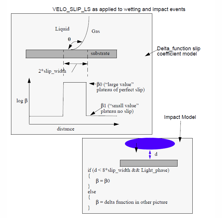
It has been found that level set interface tracking problems that involve contact or dewetting of the interfacial representation pose special problems for our numerical method. To a certain extent, we can model this type of event by making special modifications to the slipping properties of the boundary in question, however, this does not always work, especially in the case of dewetting events.

What seems to be the trouble is that we are attempting to use continuum-based models to simulate phenomena that essentially are due to molecular forces being expressed over non-molecular length scales. These length scales, while big with respect to molecules, are small with respect to our problem size. Hence, they are difficult to include in the context of reasonable mesh spacing.

The approach this boundary condition takes to inclusion of contact and dewetting phenomena is not attempt to model the finer details, but to simply note that they are due to “molecular weirdness” and thus take place outside of ordinary continuum mechanics. Therefore, there is some justification for, very briefly and in a localized area, dispensing with continuum mechanics assumption and simply imposing a contact or dewetting event. We refer to these as ADC events and will describe them in more detail later.

The parameters supplied with the card are used to determine where and when such an ADC event occurs. We have chosen to introduce a probabalistic model for this purpose. The reasoning for this comes from reflecting on the dewetting problem. If one imagines a thin sheet of fluid on a wetting substrate, it is clear that dewetting will occur eventually at some point on that sheet. Where that event occurs is somewhat random for a detached perspective. Introduction of a probability model for ADC events attempts to capture this.

Whether an ADC event occurs at an element on the sideset is determined by the following requirements:

The interface surface passes through the element.
There isn’t a contact line in the element.
The angle between the interface normal and the sideset surface normal is less than or equal to the capture angle, \(\theta_c\).
A random number in the range (0,1) determined by the standard C rand() function is less than a probability, P, given by

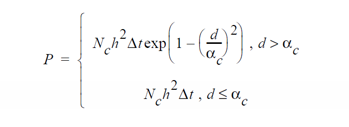
where d is the average distance of the interface to the sideset in that element, Dt is the time step size, and h is the side length of the element (Note for 2D problems \(h^2\) is replaced by h where the other dimension is assumed unity in the z direction).

Interpretation of this probability relation might take the following course. Given that the fluid interface lies within \(\alpha)c\) of the surface, the length of time necessary before and ADC event is certain to occur is given by 1/ \(N_ch^2\) . Hence, the bigger the capture rate parameter the faster this is likely to occur. The functional form for the case of d > \(\alpha_c\) is included merely to ensure that the probability drops smoothly to zero as quickly as possible. One might point out that the probability at a specific element tends towards zero as the element size decreases. Of course, in that context, the number of elements should increase in number so that the overall probability of an ADC event should not be a function of the degree of mesh refinement. A second point is that this boundary condition can be made to function as means to initiate contact without delay by simply choosing a capture rate that is large enought with respect to the current time step.

Application of an ADC event in a element that meets the preceding criteria is illustrated in the cartoon below:

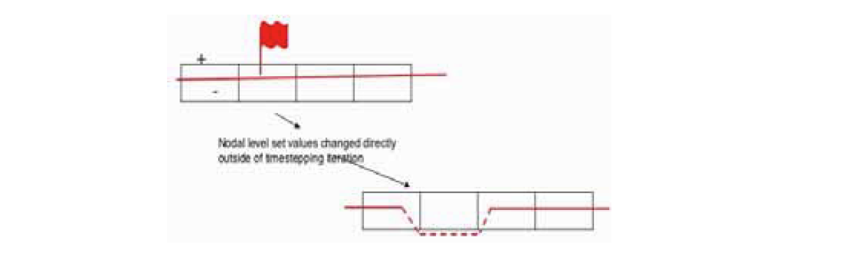
It is a simple manipulation of the level set values in that element so that the interface will follow the path indicated by the dashed curve in the lower figure. No effort is made in preservation of volume when this is done. The assumption is that these events will occur infrequently enough that this is not a significant problem. However, the user should be aware of this assumption and be careful that these events do not occur on a regular basis as then the mass loss might be more significant.

References#

No References.

LS_CA_H#

BC = LS_CA_H SS <bc_id> <float>

Description / Usage#

(WIC/SCALAR CURVATURE)

This boundary condition is used only in conjunction with level set interface tracking and the LS_CAP_CURVE embedded surface tension source term. Its function is impose a contact angle condition on that boundary.

A description of the input parameters follows:

LS_CA_H	Name of the boundary condition.
SS	Type of boundary condition (<bc_type>), where SS denotes side set in the EXODUS II database.
<bc_id>	The boundary flag identifier, an integer associated with <bc_type> that identifies the boundary location (side set in EXODUS II) in the problem domain.
<float>	A float value that is the imposed contact angle in degrees.

Examples#

An example:

BC = LS_CA_H SS 10 45.0

Technical Discussion#

The projection equation operator for solving for the curvature degree of freedom from a level set field is a Laplacian. It is standard to integrate these operators by parts but in the process one always generates a boundary integral. In this case the integral takes the form:

where \(n_w\) is the wall surface normal and \(n_{fs}\) is the normal to free surface (zero contour of the level set function ). This is a convenient event because it allows us to impose a contact angle condition on a sideset using this boundary integral by making the assignment

where \(\theta\) is the contact angle specified on the card.

The effect of this boundary condition is impose a disturbance in the curvature field near the boundary that has the effect of accelerating or decelerating the fluid near the wall in response to whether the actual contact angle is greater or less than the imposed value. Thus, over time, given no other outside influences, the contact angle should evolve from its initial value (that presumably is different than the imposed value) to the value imposed on this card. The user should expect that the contact angle will instantaneously jumped to the imposed value.

References#

No References.

LS_CAPILLARY#

BC = LS_CAPILLARY LS <integer>

Description / Usage#

(EMB/VECTOR MOMENTUM)

This boundary condition applies an “embedded” surface tension source term when solving capillary hydrodynamics problems with level set interface tracking. It can be used both when subgrid or subelement integration is being used. The surface tension value used in this boundary condition is obtained from the Surface Tension material parameter defined in the mat file.

A description of the input parameters follows:

LS_CAPILLARY	Name of the boundary condition.
LS	This string is used to indicated that this is a “boundary” condition is applied at an internal phase boundary defined by the zero contour of the level set function.
<integer>	An integer parameter than is permitted to take one of three values -1, 0, or 1. Depending upon the choice of this parameter the surface tension forces are applied to the negative phase, both phase, or the positive phase, respectively. Details are given below.

Examples#

An example:

BC = LS_CAPILLARY LS 0

Technical Discussion#

First, a warning: If subelement integration is off, make sure there is a nonzero levelset length scale or no surface forces term will be applied.

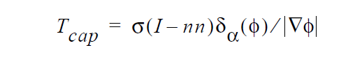
Surface tension forces at a level set representation of an interfacial boundary are applied solely via this boundary condition. An additional divergence of stress tensor term \(\Delta\) ⋅ \(T_{cap}\) is added to the fluid momentum equation. Following Jacqmin the form of this tensor is

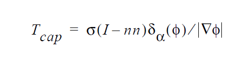
where s is the (isotropic) surface tension, I is the identity tensor, n is the vector normal to the interface and \(\zeta_a\) ( \(\phi\) ) is the smoothed Dirac delta function. The surface tension value used in this expression is obtained from the Surface Tension card found in the material file.

The actual implementation in Goma integrates the divergence term by parts so the expression that is added to the weak form of the momentum equation is:

This fact introduces the issue of integration error into the problem. As obvious above, this source term involves the non-linear Dirac delta function factor. Conventional numerical integration methods often do not offer adequate accuracy in evaluating this integral, especially if if the interface width is a fraction of the average element size. This has led to introduction the level-set-specific integration methods: subelement integration and subgrid integration. In the latter case, more integration points are clustered around the interface (in essence) to improve accuracy. The integer parameter on the card should be set to zero to signify that the surface tension forces are distributed in equal measure on both sides of the interfacial curve.

In the subelement integration case, however, an actual subelement mesh is place on each of the interface-containing elements which is made to conform to the interface curve. That is, the interface curve itself is covered by these subelement boundaries. This allows the volume integral to be collapsed into a line integral and the line integral evaluated along the subelement boundaries. This, however, introduces the problem of identifying which side of the element the surface tension forces should actually be applied to. Applying them to both simultaneously while either result in a cancellation or a doubling of the surface tension effect. For these cases, the integer parameter on this card is set to a -1 or a +1 to signify that the surface tension forces are applied to the negative or positive side of the interface curve, respectively.

References#

No References.

LS_CAP_DENNER_DIFF#

BC = LS_CAP_DENNER_DIFF LS <double>

Description / Usage#

(EMB/VECTOR MOMENTUM)

This boundary condition is expected to be paired with another boundary condition that represents the surface tension term.

e.g.

LS_CAPILLARY LS_CAP_DIV_N etc..

And should not be used with LS_CAP_HYSING

Embedded boundary condition for applying a diffusion to the level set capillary boundary condition. A time scaled diffusion term to aid with reducing spurious currents.

Not compatible with subelement integration.

A description of the input parameters follows:

LS_CAP_DENNER_DIFF	Boundary condition name
LS	Indicator that this is a level set boundary condition
<double>	Scaling of the diffusive term

Examples#

An example:

BC = LS_CAP_DENNER_DIFF LS 1.0

Technical Discussion#

Adds the following embedded boundary condition to the momentum equations:

\[- \beta \Delta t^{n+1} \int \nabla_s \mathbf{v} : (\sigma \delta_{\alpha}(\phi) \nabla_s \mathbf{u}^{n+1}) d\mathbf{x}\]

And

\[\nabla_s f = \nabla f - \mathbf{\hat{n}}^n (\mathbf{\hat{n}}^n \cdot \nabla f)\]

Where, \(\beta\) is a scaling term, \(n\) represents a timestep, and \(\mathbf{\hat{n}}\) represents the normal found from the level set function (or from the normal equations when enabled), and \(\mathbf{u}\) is the velocity.

Theory#

No Theory.

FAQs#

No FAQs.

References#

Denner, F., Evrard, F., Serfaty, R. and van Wachem, B.G., 2017. Artificial viscosity model to mitigate numerical artefacts at fluid interfaces with surface tension. Computers & Fluids, 143, pp.59-72.

LS_CAP_HYSING#

BC = LS_CAP_HYSING LS <double>

Description / Usage#

(EMB/VECTOR MOMENTUM)

Embedded boundary condition for applying a surface tension source term with level set. Has the added advantage of a time scaled diffusion term to aid with reducing spurious currents.The surface tension value used in this boundary condition is obtained from the Surface Tension material parameter defined in the mat file.

Not compatible with subelement integration.

A description of the input parameters follows:

LS_CAP_HYSING	Boundary condition name
LS	Indicator that this is a level set boundary condition
<double>	Scaling of the diffusive term

Examples#

An example:

BC = LS_CAP_HYSING LS 1.0

Technical Discussion#

Adds the following embedded boundary condition to the momentum equations:

\[- \int \nabla \mathbf{v} : (\mathbf{I} - \mathbf{\hat{n}}^n \mathbf{\hat{n}}^n) d\mathbf{x} - \beta \Delta t^{n+1} \int \nabla_s \mathbf{v} : (\sigma \delta_{\alpha}(\phi) \nabla_s \mathbf{u}^{n+1}) d\mathbf{x}\]

Where, \(\beta\) is a scaling term, \(n\) represents a timestep, and \(\mathbf{\hat{n}}\) represents the normal found from the level set function, and \(\mathbf{u}\) is the velocity.

Theory#

No Theory.

FAQs#

No FAQs.

References#

Hysing, S.R., Turek, S., Kuzmin, D., Parolini, N., Burman, E., Ganesan, S. and Tobiska, L., 2009. Quantitative benchmark computations of two‐dimensional bubble dynamics. International Journal for Numerical Methods in Fluids, 60(11), pp.1259-1288.

LS_FLOW_PRESSURE#

BC = LS_FLOW_PRESSURE LS <integer> <float1>

Description / Usage#

(EMB/VECTOR MOMENTUM)

This boundary condition applies a scalar pressure value as an “embedded” source term on the fluid momentum equation at the zero level set contour. It can be used both when subgrid or subelement integration is being used.

A description of the input parameters follows:

LS_FLOW_PRESSURE	Name of the boundary condition.
LS	This string is used to indicated that this is a “boundary” condition is applied at an internal phase boundary defined by the zero contour of the level set function.
<integer>	An integer parameter than is permitted to take one of three values -1, 0, or 1. Depending upon the choice of this parameter the pressure value is applied to the negative phase, both phase, or the positive phase, respectively. Details are given below.
<float1>	P, The constant value of pressure to be applied at the zero level set contour.

Examples#

An example:

BC = LS_FLOW_PRESSURE LS 0 1013250.0

Technical Discussion#

This boundary condition is somewhat analogous to the FLOW_PRESSURE boundary condition used quite often in ALE problems. It applies a scalar pressure at the interfacial curve as an embedded boundary condtion. It can be used in by subgrid and subelement methods. In the case of the former, a distributed volume integral of the form:

where \(\vec{n}_{fs}\) is the normal to the level set contour \(\delta_\alpha\) (\(\phi\)) and is the familiar smoothed Dirac delta function with width parameter \(\alpha\). When subelement integration is used this width parameter goes to zero and the volume integral becomes a surface integral along the zero level set contour (Note: as of Oct 2005 subelement integration is not supported for three dimensional problems).

When using this boundary condition concurrent with subgrid integration, the integer parameter that appears on the card should be consistently set to zero. This ensures the volume source will be applied symmetrically. However, when using subelement integration this integer parameter must be entire a +1 or a -1 so that the pressure force will be applied to only on side of the interface and not both which would result in cancellation. This is much the same as was seen for the LS_CAPILLARY boundary condition and the reader is referred to that card for a more detailed discussion.

References#

No References.

LS_FLUID_SOLID_CONTACT#

BC = LS_FLUID_SOLID_CONTACT LS <integer> <integer1>

Description / Usage#

(EMB/MOMENTUM)

This boundary condition applies a fluid-solid stress balance at a level set interface that is slaved to an overset mesh (see GT-026.3). It is applied as an “embedded” source term on the fluid momentum equations at the zero level set contour. NOTE: This boundary condition has been deprecated in favor of the BAAIJENS_SOLID_FLUID and BAAIJENS_FLUID_SOLID boundary conditions, as described in the memo.

A description of the input parameters follows:

LS_FLUID_SOLID_CONTACT	Name of the boundary condition.
LS	This string is used to indicated that this is a “boundary” condition is applied at an internal phase boundary defined by the zero contour of the level set function.
<integer>	An integer parameter than is permitted to take one of three values -1, 0, or 1. Depending upon the choice of this parameter the mass flux value is applied to the negative phase, both phase, or the positive phase, respectively. Details are given below.
<integer1>	Not used. Set to zero.

Technical Discussion#

We discourage use of this experimental boundary condition.

References#

No References.

LS_INLET#

BC = LS_INLET SS <bc_id>

Description / Usage#

(PCC/LEVEL SET)

This boundary condition is used to set the values of the level set function on a sideset. Most of this is done on an inlet or outlet boundary to elminate the potential for oscillations in the level set field at those points from introducing spurious interfacial (zero contours) .

A description of the input parameters follows:

LS_INLET	Name of the boundary condition.
SS	This string indicates what this boundary is applied to.
<bc_id>	An integer parameter than is permitted to take one of three values -1, 0, or 1. Depending upon the choice of this parameter the surface tension forces are applied to the negative phase, both phase, or the positive phase, respectively. Details are given below.

Examples#

An example:

BC = LS_INLET SS 10

Technical Discussion#

where s is the (isotropic) surface tension, I is the identity tensor, n is the vector normal to the interface and \(\delta_\alpha\) (\(\phi\)) is the smoothed Dirac delta function. The surface tension value used in this expression is obtained from the Surface Tension card found in the material file.

The actual implementation in Goma integrates the divergence term by parts so the expression that is added to the weak form of the momentum equation is:

References#

No References.

LS_NO_SLIP#

BC = LS_NO_SLIP PF <integer>

Description / Usage#

(EMB/VECTOR MOMENTUM)

This boundary condition is used to enforce the fluid/solid kinematic constraint for 1) overset grid applications in which 2) the solid material is assumed rigid and therefore has no internal stresses. It requires 3) a slaved phase function be defined along with 4) a vector field of Lagrange multipliers.

A description of the input parameters follows:

LS_NO_SLIP	Name of the boundary condition.
PF	This string indicates that this boundary condition is going to be applied along the zero contour of an embedded phase function (PF) field.
<integer>	This integer identifies the specific phase function field that is defining the contour. At the present time this integer should always be one.

Examples#

An example:

BC = LS_NO_SLIP PF 1

Technical Discussion#

This boundary condition is used in the context of Goma’s overset grid capability. A thorough treatment of this method is provided in the Goma document (GT-026.3) and the user is directed there. However, a brief discussion of the nature of this boundary condition is in order at this point.

The overset grid capability is used in problems in which a solid material is passing through a fluid material. The solid and fluid materials both have there own meshes. In the general problem, stresses and velocities must be transferred between each phase and therefore there is two-coupling of the respective momentum and continuity equations. This boundary condition, however, is used in the restricted case in which the solid material is assumed to be rigid and having a prescribed motion. Therefore, the coupling only proceeds in one direction : solid to fluid.

This boundary condition concerns itself with enforcing the kinematic constraint:

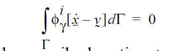
between the solid material with prescribed motion, \(\underline {\dot{x}}\) , and the fluid whose velocity is, \(\gamma\). This kinematic constraint represents a new set of equations in the model for which unknowns must be associated. In this case, we introduce a Lagrange multiplier vector field, \(\underline{\gamma}\) , at each node in the mesh. For fluid elements that do not intersect the fluid/ solid interface, these Lagrange multipliers are identically zero. They are non zero only for those fluid elements that are crossed by the fluid/solid boundary. These Lagrange multiplier fields couple the influence of the solid material on the fluid through body force terms in the fluid momentum equations of the form:

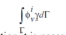
When applying this boundary condition it is necessary to include Lagrange multiplier equations equal to the number of dimensions in the problem. These are specified in the equation section of the input deck. The shape and weight functions for these fields are generally simple P0 functions. If one were to vector plot the components of the Lagrange multiplier components, you get a general picture of the force interaction field between the liquid and solid. This is sometimes informative.

A slaved phase function field is used to imprint the contour of the solid material on the liquid mesh. The zero contour of this function is then used to evaluate the above line integral. This phase function field is slaved to the solid material and is not evolved in the conventional sense. Nonetheless, a single phase function field equation must be included with the set of equations solved. In the phase function parameters section of the input deck, the user must indicate that this phase function is slaved and also must identify the sideset number of the boundary on the solid material which is the fluid/ solid interface.

References#

No References.

LS_Q#

BC = LS_Q LS <integer> <float1>

Description / Usage#

(EMB/ENERGY)

This boundary condition applies a scalar heat flux value as an “embedded” source term on the heat conservation equation at the zero level set contour. It can be used both when subgrid or subelement integration is being used.

A description of the input parameters follows:

LS_Q	Name of the boundary condition.
LS	This string is used to indicated that this is a “boundary” condition is applied at an internal phase boundary defined by the zero contour of the level set function.
<integer>	An integer parameter than is permitted to take one of three values -1, 0, or 1. Depending upon the choice of this parameter the heat flux value is applied to the negative phase, both phase, or the positive phase, respectively. Details are given below.
<float1>	q, The constant value of heat flux to be applied at the zero level set contour.

Examples#

An example:

BC = LS_Q LS 0 -1.1e-3

Technical Discussion#

This boundary condition is somewhat analogous to the QSIDE boundary condition used quite often in non-level set problems. It applies a scalar heat flux at the interfacial curve as an embedded boundary condtion. It can be used in by subgrid and subelement methods. In the case of the former, a distributed volume integral of the form:

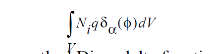
where \(\Delta\) ⋅ \(T_{cap}\) is the familiar smoothed Dirac delta function with width parameter \(\alpha\). When subelement integration is used this width parameter goes to zero and the volume integral becomes a surface integral along the zero level set contour (Note: as of Oct 2005 subelement integration is not supported for three dimensional problems).

When using this boundary condition concurrent with subgrid integration, the integer parameter that appears on the card should be consistently set to zero. This ensures the volume source will be applied symmetrically. However, when using subelement integration this integer parameter must be entire a +1 or a -1 so that the heat flux will be applied only on side of the interface and not both which would result in cancellation. This is much the same as was seen for the LS_CAPILLARY boundary condition and the reader is referred to that card for a more detailed discussion.

References#

No References.

LS_QRAD#

BC = LS_QRAD LS <integer> <float1> <float2> <float3> <float4>

Description / Usage#

(EMB/ENERGY)

This boundary condition card specifies heat flux using both convective and radiative terms. This heat flux value is applied as an “embedded” source term on the heat conservation equation at the zero level set contour (cf. BC = QRAD for ALE surfaces). It can be used both when subgrid or subelement integration is being used. The <float_list> has four parameters; definitions of the input parameters are as follows:

A description of the input parameters follows:

LS_QRAD	Name of the boundary condition.
LS	This string is used to indicated that this is a “boundary” condition is applied at an internal phase boundary defined by the zero contour of the level set function.
<integer>	An integer parameter than is permitted to take one of three values -1, 0, or 1. Depending upon the choice of this parameter the heat flux value is applied to the negative phase, both phase, or the positive phase, respectively. Details are given below.
<float1>	h, convective heat transfer coefficient.
<float2>	\(T_s\), sink temperature.
<float3>	\(\varepsilon\), total hemispherical emissivity.
<float4>	\(\sigma\), Stefan-Boltzmann constant.

Examples#

An example:

BC = LS_QRAD LS 0 10.0 273.0 0.3 5.6697e-8

Technical Discussion#

This is the level-set counterpart to BC = QRAD which is the same boundary condition applied to a parameterized mesh surface. Please see the discussion of that input record for the functional form of this boundary condition.

References#

No References.

LS_QLASER#

BC = LS_QLASER LS <integer> <float1> <float2> <float3> <float4>

Description / Usage#

(EMB/ENERGY)

This boundary condition card specifies heat flux model derived from a laser welding application. This heat flux value is applied as an “embedded” source term on the heat conservation equation at the zero level set contour (cf. BC = Q_LASER_WELD for ALE surfaces). It can be used both when subgrid or subelement integration is being used. The <float_list> has twenty-seven parameters; definitions of the input parameters are as follows:

A description of the input parameters follows:

LS_QLASER	Name of the boundary condition.
LS	This string is used to indicated that this is a “boundary” condition is applied at an internal phase boundary defined by the zero contour of the level set function.
<integer>	An integer parameter than is permitted to take one of three values -1, 0, or 1. Depending upon the choice of this parameter the heat flux value is applied to the negative phase, both phase, or the positive phase, respectively. Details are given below.
<float 1>	Nominal power of laser.
<float 2>	Power of laser at base state (simmer).
<float 3>	Base value of surface absorptivity.
<float 4>	Switch to allow tracking of normal component of liquid surface relative to laser beam axis for surface absorption (0 = OFF, 1 = ON)
<float 5>	Cutoff time for laser power.
<float 6>	Time at which laser power drops to 1/e.
<float 7>	For pulse weld, the laser power overshoot (%) of peak power at time to reach peak laser power.
<float 8>	Radius of laser beam.
<float 9>	For pulse weld, the time for laser pulse to reach peak power.
<float 10>	For pulse weld, the time for laser pulse to reach steady state in power.
<float 11>	Switch to either activate laser power distribution from beam center based on absolute distance (0) or based on radial distance in 2D plane (1).
<float 12>	Location of laser beam center (x-coordinate).
<float 13>	Location of laser beam center (y-coordinate).
<float 14>	Location of laser beam center (z-coordinate).
<float 15>	Laser beam orientation, normal to x-coordinate of body.
<float 16>	Laser beam orientation, normal to y-coordinate of body.
<float 17>	Laser beam orientation, normal to z-coordinate of body.
<float 18>	For pulse weld, spot frequency.
<float 19>	For pulse weld, total number of spots to simulate.
<float 20>	Switch to set type of weld simulation. (0=pulse weld, 1=linear continuous weld, -1=pseudo pulse weld, 2=sinusoidal continous weld)
<float 21>	For pulse weld, spacing of spots.
<float 22>	For radial traverse continuous weld, radius of beam travel.
<float 23>	Switch to activate beam shadowing for lap weld (0=OFF, 1=ON). Currently only active for ALE simulations.
<float 24>	Not active, should be set to zero.
<float 25>	For continuous weld, laser beam travel speed in xdirection (u velocity).
<float 26>	For continuous weld, laser beam travel speed in ydirection (v velocity).
<float 27>	For continuous weld, laser beam travel speed in zdirection (w velocity).

Examples#

An example:

BC = LS_QLASER LS -1 4.774648293 0 0.4 1 1 1.01 4.774648293 0.2
0.01 0.01 1 0.005 0 -0.198 -1 0 0 0.025 1 1 0.2032 -1000 0 0 0 0
0.0254

Technical Discussion#

This is the level-set counterpart to BC = Q_LASER which is the same boundary condition applied to a parameterized mesh surface. Please see the discussion of that input record for the functional form of this boundary condition.

References#

No References.

LS_RECOIL_PRESSURE#

BC = LS_RECOIL_PRESSURE LS <integer> <float1> <float2> <float3> <float4>

Description / Usage#

(EMB/VECTOR MOMENTUM)

This boundary condition card specifies heat flux model derived from a laser welding application.. This heat flux value is applied as an “embedded” source term on the heat conservation equation at the zero level set contour (cf. BC = CAP_RECOIL_PRESS for ALE surfaces). It can be used both when subgrid or subelement integration is being used. The <float_list> has seven parameters; definitions of the input parameters are as follows:

A description of the input parameters follows:

LS_RECOIL_PRESSURE	Name of the boundary condition.
LS	This string is used to indicated that this is a “boundary” condition is applied at an internal phase boundary defined by the zero contour of the level set function.
<integer>	An integer parameter than is permitted to take one of three values -1, 0, or 1. Depending upon the choice of this parameter the heat flux value is applied to the negative phase, both phase, or the positive phase, respectively. Details are given below.
<float1>	This float is currently disabled.
<float2>	This float is currently disabled.
<float3>	This float is currently disabled.
<float4>	Disabled. The boiling temperature is set to the melting point of the solidus. Use the material property “Solidus Temperature” card for this.
<float5>	This float is currently disabled.
<float6>	Conversion scale for pressure.
<float7>	Conversion scale for temperature.

Examples#

Technical Discussion#

Currently this boundary condition has coefficients for only iron and water. Several required pieces of information to use this boundary condition are not in final form, and the user can expect future changes and improvements. This boundary condition is designed for use with LS_QLASER.

References#

No References.

LS_VAPOR/LS_QVAPOR#

BC = LS_VAPOR LS <integer> <float1> <float2> <float3> <float4>

Description / Usage#

(EMB/ENERGY)

This boundary condition card specifies heat flux model derived from a laser welding application. This particular contribution accounts for the energy lost by vapor flux. This heat flux value is applied as an “embedded” source term on the heat conservation equation at the zero level set contour (cf. BC = Q_LASER_WELD for ALE surfaces). It can be used both when subgrid or subelement integration is being used. The <float_list> has four parameters; definitions of the input parameters are as follows:

A description of the input parameters follows:

LS_VAPOR	Name of the boundary condition.
LS	This string is used to indicated that this is a “boundary” condition is applied at an internal phase boundary defined by the zero contour of the level set function.
<integer>	An integer parameter than is permitted to take one of three values -1, 0, or 1. Depending upon the choice of this parameter the heat flux value is applied to the negative phase, both phase, or the positive phase, respectively. Details are given below.
<float1>	T_scale. Temperature scaling.
<float2>	q_scale. Heat flux scaling.

Examples#

An example:

BC = LS_VAPOR LS 0 273. 1.

Technical Discussion#

Currently this BC is hardwired to parameters (viz. heat capacitance, etc.) for iron. The melting point temperature is taken from the material property “Liquidus Temperature”. This boundary condition is still in the developmental stage. In using it is advisable to be working with the Sandia Goma code team.

References#

No References.

LS_YFLUX#

BC = LS_YFLUX LS <integer> <integer1> <float1> <float2>

Description / Usage#

(EMB/ENERGY)

This boundary condition applies a scalar mass flux value as an “embedded” source term on a species conservation equation at the zero level set contour. It can be used both when subgrid or subelement integration is being used.

A description of the input parameters follows:

LS_YFLUX	Name of the boundary condition.
LS	This string is used to indicated that this is a “boundary” condition is applied at an internal phase boundary defined by the zero contour of the level set function.
<integer>	An integer parameter than is permitted to take one of three values -1, 0, or 1. Depending upon the choice of this parameter the mass flux value is applied to the negative phase, both phase, or the positive phase, respectively. Details are given below.
<integer1>	w, This the species equation index to which this boundary condition is applied.
<float1>	\(h_c\), a constant value for the mass transfer coefficient at the interface.
<float2>	\(Y_c\), the “bulk” concentration of species used in conjunction with the mass transfer coefficient to compute the mass flux.

Examples#

An example:

BC = LS_YFLUX LS 0 0 1.e-2 0.75

Technical Discussion#

This boundary condition is somewhat analogous to the YFLUX boundary condition used quite often in non-level set problems to apply a scalar species flux at a at boundary defined by a side set. It applies a scalar mass transfer flux at the interfacial curve as an embedded boundary condtion. It can be used in by subgrid and subelement methods. In the case of the former, a distributed volume integral of the form:

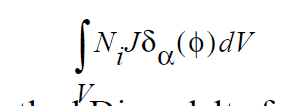
where \(\delta_\alpha\) (\(\phi\)) is the familiar smoothed Dirac delta function with width parameter \(\alpha\) and the mass flux , J, is given by the typical relation:

When subelement integration is used this width parameter goes to zero and the volume integral becomes a surface integral along the zero level set contour (Note: as of Oct 2005 subelement integration is not supported for three dimensional problems).

When using this boundary condition concurrent with subgrid integration, the integer parameter that appears on the card should be consistently set to zero. This ensures the volume source will be applied symmetrically. However, when using subelement integration this integer parameter must be entire a +1 or a -1 so that the mass flux will be applied only on side of the interface and not both which would result in cancellation. This is much the same as was seen for the LS_CAPILLARY boundary condition and the reader is referred to that card for a more detailed discussion.

References#

No References.

SHARP_BLAKE_VELOCITY#

BC = SHARP_BLAKE_VELOCITY SS <bc_id> <floatlist

Description / Usage#

(WIC/VECTOR MOMENTUM)

This boundary condition is used to induce fluid velocity at a wetting line when using Level Set Interface Tracking. Its formulation is identical to the WETTING_SPEED_BLAKE boundary condition, but it is applied as a single point source on the boundary instead of a distributed stress.

This boundary condition can only be used for two-dimensional problems.

A description of the input parameters follows:

SHARP_BLAKE_VELOCITY	Name of the boundary condition.
SS	Type of boundary condition (<bc_type>), where SS denotes side set in the EXODUS II database.
<bc_id>	The boundary flag identifier, an integer associated with <bc_type> that identifies the boundary location (side set in EXODUS II) in the problem domain.
<float1>	\(\theta_s\), the static contact angle in degress.
<float2>	V_0 is a pre-exponential velocity factor (see functional form below).
<float3>	g is a thermally scaled surface tension, i.e. \(\sigma\) /2nkT.
<float4>	\(\beta\), slip coefficient.
<float5>	\(t_{relax}\) is a relaxation time which can be used to smooth the imposed contact point velocity for transient problems. Set to zero for no smoothing.
<float6>	\(V_{old}\) is an initial velocity used in velocity smoothing for transient problems. Set to zero when smoothing is not used.

Examples#

An example:

BC = SHARP_BLAKE_VELOCITY SS 10 30.0 0.1 8. 0.001 0   0

Technical Discussion#

The implementation for this wetting condition is identical to that of SHARP_WETLIN_VELOCITY, but the wetting velocity dependence is different. Because the wetting stress is not applied at a point, it is most appropriate for use when using subelement integration which similarly collapses the surface tension sources associated with the interface onto the interfacial curve.

Note also that this boundary condition is strictly for use with two-dimensional problems. Attempting to apply it to a three dimensional problem will result in an error message.

Theory#

Derivation of the force condition for this boundary condition starts with a simple relation for wetting line velocity

Note that the convention for contact angles in this relation is that values of θ near to zero indicate a high degree of wetting and values of θ near 180 ° indicate the opposite. This is mapped to a stress value by analogy with Navier’s slip relation and has the following form when the velocity smoothing is not used,

References#

No References.

SHARP_CA_2D#

BC = SHARP_CA_2D SS <bc_id> <float>

Description / Usage#

(WIC/VECTOR MOMENTUM)

This boundary condition is used to impose a contact angle on a boundary when using Level Set Interface Tracking. It can only be used for two-dimensional problems.

A description of the input parameters follows:

FILL_CA	Name of the boundary condition.
SS	Type of boundary condition (<bc_type>), where SS denotes side set in the EXODUS II database.
<bc_id>	The boundary flag identifier, an integer associated with <bc_type> that identifies the boundary location (side set in EXODUS II) in the problem domain.
<float>	\(\theta\), the contact angle imposed, in degrees.

Examples#

An example:

BC = SHARP_CA_2D SS 10 30.0

Technical Discussion#

This boundary condition must be used in conjunction with the VELO_SLIP_FILL or VELO_SLIP_LS boundary condition. These latter conditions permits the fluid to slip in the vicinity of the contact line. The SHARP_CA_2D acts by imposing a force on the momentum equation. The size of this force is more or less in proportion between the actual contact angle on the boundary and the value specified on the card and scales directly with the applied surface tension material parameter. In this manner, it is very similar to the FILL_CA boundary condition.

The manner in which is applied differs. In this case, the applied force is not distributed around the contact line using a smooth delta function weighting in a weak integrated context, but instead the delta function is used to resolve the line integral and the force is applied directly at a point on the sideset set. Hence, this boundary condition is most appropriate for use in conjunction with subelement integration which performs a similar transformation of the volumetric surface tension source terms. Further, the logic use to identify the point of application on the boundary functions only in twodimensions. Hence, this boundary condition is stricly limited to two-dimensional problems.

References#

No References.

SHARP_COX_VELOCITY#

BC = SHARP_COX_VELOCITY SS <bc_id> <floatlist

Description / Usage#

(WIC/VECTOR MOMENTUM)

This boundary condition is used to induce fluid velocity at a wetting line when using Level Set Interface Tracking. Its formulation is identical to the WETTING_SPEED_COX boundary condition, but it is applied as a single point source on the boundary instead of a distributed stress.

This boundary condition can only be used for two-dimensional problems.

A description of the input parameters follows:

SHARP_COX_VELOCITY	Name of the boundary condition.
SS	Type of boundary condition (<bc_type>), where SS denotes side set in the EXODUS II database.
<bc_id>	The boundary flag identifier, an integer associated with <bc_type> that identifies the boundary location (side set in EXODUS II) in the problem domain.
<float1>	\(\theta_s\), the static contact angle in degress.
<float2>	\(\sigma\) is the surface tension.
<float3>	\(\varepsilon_s\) is the dimensionless slip length, i.e. the ratio of the slip length to the characteristic length scale of the macroscopic flow.
<float4>	\(\beta\), slip coefficient.
<float5>	\(t_{relax}\) is a relaxation time which can be used to smooth the imposed contact point velocity for transient problems. Set to zero for no smoothing.
<float6>	\(V_{old}\) is an initial velocity used in velocity smoothing for transient problems. Set to zero when smoothing is not used.

Examples#

An example:

BC = SHARP_COX_VELOCITY SS 10 30.0 72.0 0.01 0.1   0   0

Technical Discussion#

Note also that this boundary condition is strictly for use with two-dimensional problems. Attempting to apply it to a three dimensional problem will result in an error message.

Theory#

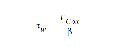
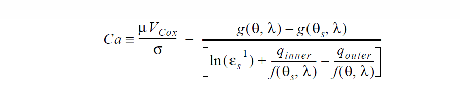
Derivation of the force condition for this boundary condition starts with a relation for wetting line velocity

where \(V_{Cox}\) is computed from the Cox hydrodynamic wetting theory;

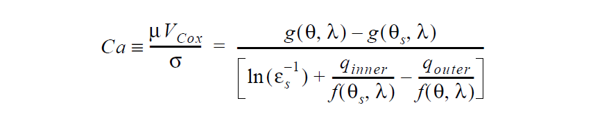
See VELO_THETA_COX for details of the Cox functions f and g. Note that the parameters \(\lambda\), \(q_{inner}\), and \(q_{outer}\) are currently not accessible from the input card and are hard-set to zero. \(\lambda\) is the ratio of gas viscosity to liquid viscosity whereas \(q_{inner}\) and \(q_{outer}\) represent influences from the inner and outer flow regions.

Note that the convention for contact angles in this relation is that values of θ near to zero indicate a high degree of wetting and values of \(\theta\) near 180 ° indicate the opposite. This is mapped to a stress value by analogy with Navier’s slip relation and has the following form when the velocity smoothing is not used,

The Cox wetting velocity requires evaluation of integrals for the function g(\(\theta\), \(\lambda\)) which is currently done numerically using 10-point Gaussian quadrature. As such the evaluation of the integrals is expected to become inaccurate as either \(\theta_s\) tends toward zero or \(\theta\) tends toward 180 degrees. Note that the integrand becomes singular as \(\theta\) tends toward 0 or 180 degrees.

References#

No References.

SHARP_HOFFMAN_VELOCITY#

BC = SHARP_HOFFMAN_VELOCITY SS <bc_id> <floatlist

Description / Usage#

(WIC/VECTOR MOMENTUM)

This boundary condition is used to induce fluid velocity at a wetting line when using Level Set Interface Tracking. Its formulation is identical to the WETTING_SPEED_HOFFMAN boundary condition, but it is applied as a single point source on the boundary instead of a distributed stress.

This boundary condition can only be used for two-dimensional problems.

A description of the input parameters follows:

SHARP_HOFFMAN_VELOCITY	Name of the boundary condition.
SS	Type of boundary condition (<bc_type>), where SS denotes side set in the EXODUS II database.
<bc_id>	The boundary flag identifier, an integer associated with <bc_type> that identifies the boundary location (side set in EXODUS II) in the problem domain.
<float1>	\(\theta_s\), the static contact angle in degress.
<float2>	\(\sigma\) is the surface tension.
<float3>	\(\beta\), slip coefficient.
<float4>	\(t_{relax}\) is a relaxation time which can be used to smooth the imposed contact point velocity for transient problems. Set to zero for no smoothing.
<float5>	\(V_{old}\) is an initial velocity used in velocity smoothing for transient problems. Set to zero when smoothing is not used.

Examples#

An example:

BC = SHARP_HOFFMAN_VELOCITY SS 10 30.0 72.0 0.1   0   0

Technical Discussion#

Note also that this boundary condition is strictly for use with two-dimensional problems. Attempting to apply it to a three dimensional problem will result in an error message.

Theory#

Derivation of the force condition for this boundary condition starts with a relation for wetting line velocity

where \(V_{Hoffman}\) is computed from the Hoffman correlation;

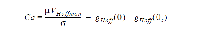
See VELO_THETA_HOFFMAN for details of the Hoffman function g. Note that the convention for contact angles in this relation is that values of \(\theta\) near to zero indicate a high degree of wetting and values of \(\theta\) near 180 ° indicate the opposite. This is mapped to a stress value by analogy with Navier’s slip relation and has the following form when the velocity smoothing is not used,

Because the Hoffman functions are implicit, iteration is required in the determination of the wetting velocity. As a result, for very high Capillary numbers, i.e. > \(10^6\), the iteration procedure in Goma may need to be modified.

References#

No References.

SHARP_WETLIN_VELOCITY#

BC = SHARP_WETLIN_VELOCITY SS <bc_id> <floatlist

Description / Usage#

(WIC/VECTOR MOMENTUM)

This boundary condition is used to induce fluid velocity at a wetting line when using Level Set Interface Tracking. Its formulation is identical to the WETTING_SPEED_LINEAR boundary condition, but it is applied as a single point source on the boundary instead of a distributed stress.

This boundary condition can only be used for two-dimensional problems.

A description of the input parameters follows:

SHARP_WETLIN_VELOCITY	Name of the boundary condition.
SS	Type of boundary condition (<bc_type>), where SS denotes side set in the EXODUS II database.
<bc_id>	The boundary flag identifier, an integer associated with <bc_type> that identifies the boundary location (side set in EXODUS II) in the problem domain.
<float1>	\(\theta_s\), the static contact angle in degress.
<float2>	\(c_T\), proportionality constant as defined below
<float3>	Currently not used.
<float4>	\(\beta\), slip coefficient.

Examples#

An example:

BC = SHARP_WETLIN_VELOCITY SS 10 30.0 0.1 0. 0.001

Technical Discussion#

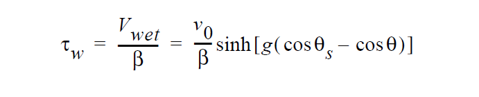
As noted above, this boundary condition imposes the same wetting stress dependence as the WETTING_SPEED_LINEAR boundary condition. However, its application in the FEM context is different. Instead of the wetting stress, \(\tau_w\), being applied according to the formula:

as is the case for the WETTING_SPEED_LINEAR condition, the Dirac function is used to remove the integral and replace it with a point stress at the location where \(\phi\) = 0 on the boundary. Designating this point as \(X_{cl}\), the vector applied to the momentum equation is given by

Because the wetting stress is not applied at a point, it is most appropriate for use when using subelement integration which similarly collapses the surface tension sources associated with the interface onto the interfacial curve. Note that this method of application is identical to the SHARP_CA_2D boundary condition discussed elsewhere.

Note also that this boundary condition is strictly for use with two-dimensional problems. Attempting to apply it to a three dimensional problem will result in an error message.

Theory#

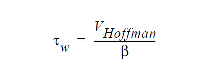
Derivation of the force condition for this boundary condition starts with a simple relation for wetting line velocity

Note that the convention for contact angles in this relation is that values of \(\theta\) near to zero indicate a high degree of wetting and values of \(\theta\) near 180 ° indicate the opposite. This is mapped to a stress value by analogy with Navier’s slip relation,

It should be noted that there is no distinction for this model in the function of \(\beta\) or \(c_T\). The two parameters are interchangeable. In non-linear models, (see WETTING_SPEED_BLAKE) this is no longer true.

References#

No References.

WETTING_SPEED_BLAKE#

BC = WETTING_SPEED_BLAKE SS <bc_id> <floatlist>

Description / Usage#

(WIC/VECTOR MOMENTUM)

This boundary condition is used to induce fluid velocity at a wetting line when using Level Set Interface Tracking. It implements a version of the Blake-DeConinck molecular-kinetic theory wetting model.

A description of the input parameters follows:

WETTING_SPEED_BLAKE	Name of the boundary condition.
SS	Type of boundary condition (<bc_type>), where SS denotes side set in the EXODUS II database.
<bc_id>	The boundary flag identifier, an integer associated with <bc_type> that identifies the boundary location (side set in EXODUS II) in the problem domain.
<float1>	\(\theta_s\), the static contact angle, degrees .
<float2>	V_0 is a pre-exponential velocity factor (see functional form below).
<float3>	g is a thermally scaled surface tension, i.e. \(\sigma\)/2nkT.
<float4>	w, width of interfacial region near contact line. Defaults to level set length scale if zero or less.
<float5>	\(\beta\), slip coefficient.
<float6>	currently not used.
<float7>	currently not used.
<float8>	currently not used.

Examples#

An example:

BC = WETTING_SPEED_BLAKE SS 10 30.0 20.1 7.0 0.   0.001 0. 0. 0.

Technical Discussion#

The implementation for this wetting condition is identical to that of WETTING_SPEED_LINEAR, but the wetting velocity dependence is different.

Note that it is a requirement that when using this boundary condition that slip to some extent be allowed on this boundary. This is most often done by applying a VELO_SLIP_LS boundary condition in conjunction with this boundary condition. In addition, a no penetration condition on the velocity is need in either the form of a Dirichlet condition or a VELO_NORMAL condition. It is important to note that the slipping condition need not relax the no slip requirement completely. In fact, its parameters should be set so that no slip is for the most part satisfied on the boundary in regions away from the contact line. Near the contact line however the parameters in the slip condition and the WETTING_SPEED_BLAKE condition need to be fixed so that appreciable fluid velocity is induced. This is a trial and error process at the current time.

Theory#

Derivation of this boundary condition starts with a relation propose by Blake and DeConinck for wetting line motion

This is mapped to a stress value by analogy with Navier’s slip relation,

This relation contrasts with the “linear” relation applied by the WETTING_SPEED_LINEAR relation in that the rate of change of the wetting velocity with the contact angle decreases as the wetting angle deviates more and more from its static value. This is more consisten with physical behaviors that the linear model.

In point of fact this condition is a vector condition so this scalar stress value multiplies the unit vector tangent to the surface and normal to the contact line, \(\vec{t}\) . This stress is then weighted by smooth Dirac function to restrict its location to being near the interface, weighted by a FEM shape function, integrated over the boundary sideset and added to the fluid momentum equation for the corresponding node j, vis:

References#

No References.

WETTING_SPEED_COX#

BC = WETTING_SPEED_COX SS <bc_id> <floatlist

Description / Usage#

(WIC/VECTOR MOMENTUM)

This boundary condition is used to induce fluid velocity at a wetting line when using Level Set Interface Tracking. It implements a version of the Cox hydrodynamic model of wetting.

A description of the input parameters follows:

WETTING_SPEED_COX	Name of the boundary condition.
SS	Type of boundary condition (<bc_type>), where SS denotes side set in the EXODUS II database.
<bc_id>	The boundary flag identifier, an integer associated with <bc_type> that identifies the boundary location (side set in EXODUS II) in the problem domain.
<float1>	\(\theta_s\), the static contact angle, degrees.
<float2>	\(\varepsilon_s\) is the dimensionless slip length, i.e. the ratio of the slip length to the characteristic length scale of the macroscopic flow.
<float3>	\(\sigma\) is the surface tension.
<float4>	w ,width of interfacial region near contact line. Defaults to level set length scale if zero or less.
<float5>	\(\beta\), slip coefficient.
<float6>	currently not used.
<float7>	currently not used.
<float8>	currently not used.

Examples#

An example:

BC = WETTING_SPEED_COX SS 10 30.0 0.01 72.0 0.   0.001 0. 0. 0.

Technical Discussion#

The implementation for this wetting condition is identical to that of WETTING_SPEED_LINEAR, but the wetting velocity dependence is different.

Theory#

Derivation of this boundary condition starts with a relation that represents the Cox hydrodynamic wetting model

This relation contrasts with the “linear” relation applied by the WETTING_SPEED_LINEAR relation in that more consistent physical behavior should result.

References#

No References.

WETTING_SPEED_HOFFMAN#

BC = WETTING_SPEED_HOFFMAN SS <bc_id> <floatlist

Description / Usage#

(WIC/VECTOR MOMENTUM)

This boundary condition is used to induce fluid velocity at a wetting line when using Level Set Interface Tracking. It implements a version of the Hoffman wetting correlation.

A description of the input parameters follows:

WETTING_SPEED_HOFFMAN	Name of the boundary condition.
SS	Type of boundary condition (<bc_type>), where SS denotes side set in the EXODUS II database.
<bc_id>	The boundary flag identifier, an integer associated with <bc_type> that identifies the boundary location (side set in EXODUS II) in the problem domain.
<float1>	\(\theta_s\), the static contact angle, degrees .
<float2>	currently not used.
<float3>	\(\sigma\) is the surface tension.
<float4>	w, width of interfacial region near contact line. Defaults to level set length scale if zero or less.
<float5>	\(\beta\), slip coefficient.
<float6>	currently not used.
<float7>	currently not used.
<float8>	currently not used.

Examples#

An example:

BC = WETTING_SPEED_HOFFMAN SS 10 30.0 0 72.0   0. 0.001 0. 0. 0.

Technical Discussion#

The implementation for this wetting condition is identical to that of WETTING_SPEED_LINEAR, but the wetting velocity dependence is different.

Theory#

Derivation of this boundary condition starts with a relation that represents the Hoffman wetting correlation

This relation contrasts with the “linear” relation applied by the WETTING_SPEED_LINEAR relation in that more consistent physical behavior should result.

References#

Stephan F. Kistler 1993. “Hydrodynamics of Wetting” in Wettability, edited by John Berg, Surfactant Science Series, 49, Marcel Dekker, NewYork, NY, pp. 311-429.

WETTING_SPEED_LINEAR#

BC = WETTING_SPEED_LINEAR SS <bc_id> <floatlist

Description / Usage#

(WIC/VECTOR MOMENTUM)

This boundary condition is used to induce fluid velocity at a wetting line when using Level Set Interface Tracking.

A description of the input parameters follows:

WETTING_SPEED_LINEAR	Name of the boundary condition.
SS	Type of boundary condition (<bc_type>), where SS denotes side set in the EXODUS II database.
<bc_id>	The boundary flag identifier, an integer associated with <bc_type> that identifies the boundary location (side set in EXODUS II) in the problem domain.
<float1>	\(\theta_s\), the static contact angle in degrees.
<float2>	\(c_T\), proportionality constant as defined below
<float3>	w ,width of interfacial region near contact line. Defaults to level set length scale if zero or less (L).
<float4>	\(\beta\), slip coefficient.
<float5>	currently not used.
<float6>	currently not used.
<float7>	currently not used.

Examples#

An example:

BC = WETTING_SPEED_LINEAR SS 10 30.0 0.1 0. 0.001 0. 0. 0.

Technical Discussion#

The prescence of wetting or contact lines in problems using level set interface tracking introduces the problem of modeling the motion of the wetting line. This boundary condition presents one potential means for doing this. It adds a wall stress value at the boundary in a region near to the wetting line (this is set with the Level Set Length Scale discussed previously). This wall stress value depends upon the deviation of the apparent contact angle determined from the level set function and a set static contact angle. The bigger the deviation in principle the bigger the induced stress. The stress is modeled by analogy with Navier’s slip relation (with slip coefficient \(\beta\)). The stress will induce a fluid velocity at the boundary which it is hoped will move the contact line at a velocity that is consistent with the rest of the flow.

An important note is that it is a requirement that when using this boundary condition that slip to some extent be allowed on this boundary. This is most often done by applying a VELO_SLIP_LS boundary condition in conjunction with this boundary condition. In addition, a no penetration condition on the velocity is need in either the form of a Dirichlet condition or a VELO_NORMAL condition. It is important to note that the slipping condition need not relax the no slip requirement completely. In fact, its parameters should be set so that no slip is for the most part satisfied on the boundary in regions away from the contact line. Near the contact line however the parameters in the slip condition and the WETTING_SPEED_LINEAR condition need to be fixed so that appreciable fluid velocity is induced. This is a trial and error process at the current time.

Theory#

Derivation of this boundary condition starts with a simple relation for wetting line velocity

References#

No References.

LINEAR_WETTING_SIC#

BC = LINEAR_WETTING_SIC SS <bc_id> <floatlist>

Description / Usage#

(SIC/VECTOR MOMENTUM)

This boundary condition is used to induce fluid velocity at a wetting line when using Level Set Interface Tracking. It is an alternative to the WETTING_SPEED_LINEAR BC which does not require the VELO_SLIP_LS or VELO_SLIP_FILL BC’s on the wetting boundary.

A description of the input parameters follows:

LINEAR_WETTING_SIC	Name of the boundary condition.
SS	Type of boundary condition (<bc_type>), where SS denotes side set in the EXODUS II database.
<bc_id>	The boundary flag identifier, an integer associated with <bc_type> that identifies the boundary location (side set in EXODUS II) in the problem domain.
<float1>	\(\theta_s\), the static contact angle in degress.
<float2>	\(c_T\), proportionality constant as defined below.
<float3>	w, width of interfacial region near contact line. Defaults to level set length scale if zero or less (L).
<float4>	\(\beta\), slip coefficient.
<float5>	\(v_{sx}\), x-component of substrate velocity.
<float6>	\(v_{sy}\), y-component of substrate velocity.
<float7>	\(v_{sz}\), z-component of substrate velocity.
<float8>	\(\tau\), stability parameter.

Examples#

Here is an example card:

BC = LINEAR_WETTING_SIC SS 10 30.0 0.1 0. 0.001 0. 0. 0. 0.

Technical Discussion#

This boundary condition is an additional means to impose a wetting line velocity at the contact line for level set interface tracking problems. The boundary condition uses a form of the Navier-Stokes slip condition to impose a boundary shear stress term to the momentum equation:

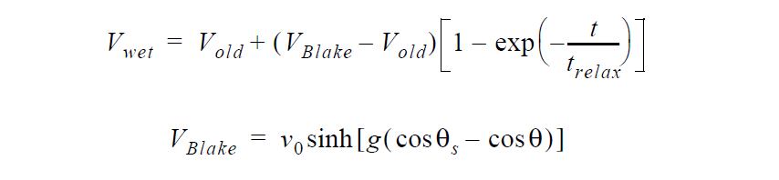
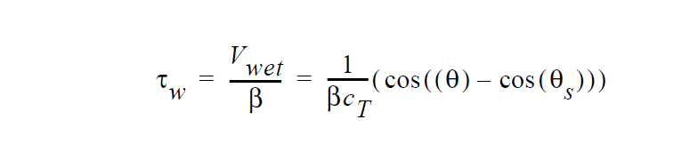
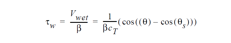
where \(\vec{n}\) and \(\vec{t}\) are the normal and tangent boundary vectors, respectively, \(\beta\) is the “slipping” parameter which in this context is used actually as a penalty parameter, \(\vec{v}_s\) is the substrate velocity, \(\tau\) is a stabilization parameter, \(V_{wet}\) is the wetting velocity given by the following relation

The masking function f(F) is given by the following relation as well:

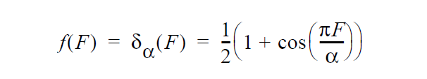
where \(\alpha\) is the width of the interfacial region near the contact line itself. It has the effect of “turning off” the wetting velocity at points on the boundary away from the interface.

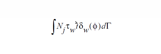
This constraint is then introduced into the fluid momentum equation via the weak natural boundary condition term:

When applying this boundary condition, the user should choose a value for \(\beta\) which is relatively small. Its size is dictated by the requirement that away from the interface this boundary condition should be imposing a no-slip condition on the fluid velocity. Conversely, in the vicinity of the wetting line this boundary condition will impose the wetting velocity as computed from the preceding equation.

This boundary condition probably should be used in conjunction with a no penetration boundary condition, for example, a VELO_NORMAL condition on the same sideset or potentially a Dirichlet condition on velocity if the geometry permits this. In theory, this boundary condition can be used to impose no penetration as well, but this will require a very small value for \(\beta\). The user should experiment with this.

The stability parameter, \(\tau\), as requires commentary. It is helpful to imagine that this parameter introduces a certain amount of inertia to motion of the contact line. With this term active (non-zero value for \(\tau\)), large changes of the contact line velocity with time are restricted. This can be quite helpful during startup when the intial contact angle is often very different from its equilibrium value and there can be very large velocities generated as a result. These may in turn lead to low time step size and other numerical problems.

Although every situation is different, one should choose values for \(\tau\) which are on the order of 1 to 10 times the starting time step size of the simulation. One should also recognize that this term is not consistent from a physical standpoint and therefore one should endeavor to keep \(\tau\) as small as possible if not in fact equal to zero.

References#

No References.

BLAKE_DIRICHLET#

BC = BLAKE_DIRICHLET SS <bc_id> <floatlist>

Description / Usage#

(SIC/VECTOR MOMENTUM)

This boundary condition is used to induce fluid velocity at a wetting line when using Level Set Interface Tracking. It is an alternative to the WETTING_SPEED_BLAKE BC which does not require the VELO_SLIP_LS or VELO_SLIP_FILL BC’s on the wetting boundary. It uses a Blake-DeConninck relationship between apparent contact angle and wetting velocity. As the name implies, this boundary condition differs from WETTING_SPEED_BLAKE in that wetting velocity is in a strong fashion on the wetting boundary.

A description of the input parameters follows:

BLAKE_DIRICHLET	Name of the boundary condition.
SS	Type of boundary condition (<bc_type>), where SS denotes side set in the EXODUS II database.
<bc_id>	The boundary flag identifier, an integer associated with <bc_type> that identifies the boundary location (side set in EXODUS II) in the problem domain.
<float1>	\(\theta_s\), the static contact angle in degrees.
<float2>	\(V_0\) is a pre-exponential velocity factor (see functional form below). (L/T)
<float3>	g is a thermally scaled surface tension, i.e. \(\sigma\)/2nkT. Note that this parameter will be multiplied by the surface tension supplied in the material file when its used in the wetting velocity relation.
<float4>	w, is the width of the interface wetting region. It defaults to the level set length scale if zero of less.
<float5>	\(\tau\), stability parameter (T).
<float6>	\(v_{sx}\), x-component of substrate velocity.
<float7>	\(v_{sy}\), y-component of substrate velocity (L/T).
<float8>	\(v_{sz}\), z-component of substrate velocity.

Examples#

Here is an example card:

BC = BLAKE_DIRICHLET SS 10 30.0 20.1 7.0 0.0 0.001 0. 0. 0.

Technical Discussion#

This boundary condition is an additional means to impose a wetting line velocity at the contact line for level set interface tracking problems. It is related to the WETTING_SPEED_BLAKE condition in that it uses the same Blake-DeConninck relationship between contact angle and wetting speed, but it applies this relation to the computational setting in a different way.

In this case, the following vector constraint is added to fluid momentum equation on the sideset to which this boundary condition is applied:

The factor P is a large penalty parameter which swamps any contributions from the volumetric momentum equations. Thus, the velocity, \(\sec{v}\) , on this boundary will be set solely by the preceding constraint. In this sense, it is a Dirichlet condition (strictly speaking, Dirichlet conditions involve direct substitution of nodal degrees-of-freedom with corresponding elimination of its equation from the matrix which this boundary condition does NOT do).

In the preceding, the vector \(\sec{t}\), is a tangent vector to the surface and always points in the same direction of the level set gradient on the boundary (that is, from negative to positive). In three dimensions, \(\sec{t}\) will also be normal to the contact line curve as it intersects the surface itself.

The masking function, f(\(\phi\);w) , is used to limit the application of the wetting line velocity to only that region of the boundary that is the in immediate vicinity of the contact line. We use a simple “hat” function:

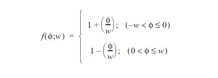
Needless to say, f(\(\phi\);w) is identically zero for level set values outside the interval (-w,*w*).

The stabilization term, -\(\tau\) \(\frac{∂v}{∂t}\) , is intended to introduce something like inertia to the wetting line. That is to say, it’s primary effect is to limit the rate of change of the wetting line velocity to “reasonable” values. The \(\tau\) parameter should be chosen to be on the order of the smallest anticipated time step size in the problem. Setting it at zero, of course, will remove this term entirely.

In general, this boundary condition can be used to exclusively to set both the wetting speed velocity and the no slip requirement on the indicated sideset set. This would also include the no penetration requirement. The user may, however, find it advantageous to apply this constraint directly with the VELO_NORMAL condition on the same side set.

An additional note is that the “scaled viscosity” parameter g will be multiplied by the surface tension value supplied with Surface Tension card in the material file.

Theory#

The wetting speed model for this boundary condition is the same used by the WETTING_SPEED_BLAKE card:

References#

T. D. Blake and J. De Coninck 2002. “The Influence of Solid-Liquid Interactions on Dynamic Wetting”, Advances in Colloid and Interface Science, 96, 21-36.

COX_DIRICHLET#

BC = COX_DIRICHLET SS <bc_id> <floatlist>

Description / Usage#

(SIC/VECTOR MOMENTUM)

This boundary condition is used to induce fluid velocity at a wetting line when using Level Set Interface Tracking. It is an alternative to the WETTING_SPEED_COX which does not require the VELO_SLIP_LS or VELO_SLIP_FILL BC’s on the wetting boundary. It implements a version of the Cox hydrodynamic model of wetting (see below). As the name implies, this boundary condition differs from WETTING_SPEED_COX in that wetting velocity is applied in a strong fashion on the wetting boundary.

A description of the input parameters follows:

COX_DIRICHLET	Name of the boundary condition.
SS	Type of boundary condition (<bc_type>), where SS denotes side set in the EXODUS II database.
<bc_id>	The boundary flag identifier, an integer associated with <bc_type> that identifies the boundary location (side set in EXODUS II) in the problem domain.
<float1>	\(\theta_s\), the static contact angle in degress.
<float2>	\(\varepsilon_s\) is the dimensionless slip length, i.e. the ratio of the slip length to the characteristic length scale of the macroscopic flow. (L)
<float3>	\(\sigma\) is the surface tension. Note this value will be scaled by the surface tension value supplied in the material file.(F/L)
<float4>	w, is the width of the interface wetting region. It defaults to the level set length scale if zero of less (L).
<float5>	\(\tau\), stability parameter (T).
<float6>	\(v_{sx}\), x-component of substrate velocity.
<float7>	\(v_{sy}\), y-component of substrate velocity (L/T).
<float8>	\(v_{sz}\), z-component of substrate velocity.

Examples#

Here is an example card:

BC = COX_DIRICHLET SS 10 30.0 0.01 72.0   0. 0.001 0. 0. 0.

Technical Discussion#

This boundary condition is applied in exactly the same manner as the BLAKE_DIRICHLET boundary condition. The only substantial difference is the model used to derive the wetting speeds relation to the local apparent contact angle. The reader is referred to the BLAKE_DIRICHLET section of the manual for further reference.

Theory#

This boundary condition uses this relation that represents the Cox hydrodynamic wetting model

References#

Stephan F. Kistler 1993. “Hydrodynamics of Wetting” in Wettability, edited by John Berg, Surfactant Science Series, 49, Marcel Dekker, NewYork, NY, pp. 311-429.

HOFFMAN_DIRICHLET#

BC = HOFFMAN_DIRICHLET SS <bc_id> <floatlist>

Description / Usage#

(SIC/VECTOR MOMENTUM)

This boundary condition is used to induce fluid velocity at a wetting line when using Level Set Interface Tracking. It is an alternative to the WETTING_SPEED_HOFFMAN boundary condition which does not require the VELO_SLIP_LS or VELO_SLIP_FILL BC’s on the wetting boundary. As the name implies, this boundary condition differs from WETTING_SPEED_HOFFMAN in that wetting velocity is in a strong fashion on the wetting boundary.

A description of the input parameters follows:

HOFFMAN_DIRICHLET	Name of the boundary condition.
SS	Type of boundary condition (<bc_type>), where SS denotes side set in the EXODUS II database.
<bc_id>	The boundary flag identifier, an integer associated with <bc_type> that identifies the boundary location (side set in EXODUS II) in the problem domain.
<float1>	\(\theta_s\), the static contact angle in degress.
<float2>	not used.
<float3>	\(\sigma\), the surface tension. Note that this parameter will be scaled by the surface tension value supplied in the material file. (F/L)
<float4>	w, is the width of the interface wetting region. It defaults to the level set length scale if zero of less.
<float5>	\(\tau\), stability parameter (T).
<float6>	\(v_{sx}\), x-component of substrate velocity.
<float7>	\(v_{sy}\), y-component of substrate velocity (L/T).
<float8>	\(v_{sz}\), z-component of substrate velocity.

Examples#

Here is an example card:

BC = HOFFMAN_DIRICHLET SS 10 30.0 0 72.0 0.0 0.001 0. 0. 0.

Technical Discussion#

The technical details of the application of this boundary differ not at all from those described for the BLAKE_DIRICHLET boundary condition. The user is referred to that section for further details. This boundary condition differs only in the model used to determine the wetting velocity. This is described below and in the VELO_THETA_HOFFMAN card.

Theory#

Derivation of this boundary condition starts with a relation that represents the Hoffman wetting correlation

References#

Stephan F. Kistler 1993. “Hydrodynamics of Wetting” in Wettability, edited by John Berg, Surfactant Science Series, 49, Marcel Dekker, NewYork, NY, pp. 311-429.

VELO_SLIP_LS#

BC = VELO_SLIP_LS SS <bc_id> <float_list>

Description / Usage#

(WIC/VECTOR MOMENTUM)

This boundary condition is applied only in problems involving embedded interface tracking, that is, level set or volume of fluid. The boundary condition serves two major purposes: first to allow for slip in the vicinity of a moving contact line and second to facilitate impact of a dense fluid on a substrate, displacing a less dense fluid (e.g. water drop and air displacement). . Elsewhere, this boundary condition enforces a no-slip condition between fluid and substrate. A more detailed description is given below.

This boundary condition is most often used in conjunction with the FILL_CA, WETTING_SPEED_LINEAR, or WETTING_SPEED_BLAKE boundary conditions. These apply forces to contact lines in order to simulate wetting line motion. These forces are applied in a weak sense to the same regions near the interface so it is necessary to use VELO_SLIP_LS with a large slipping coefficient so that effectively no-slip is relaxed completely near the interface.

Definitions of the input parameters are as follows:

VELO_SLIP_LS	Name of the boundary condition.
SS	Type of boundary condition (<bc_type>), where SS denotes side set in the EXODUS II database.
<bc_id>	The boundary flag identifier, an integer associated with <bc_type> that identifies the boundary location (side set in EXODUS II) in the problem domain.
<float1>	alpha, or slip_width, a characteristic length scale around the contact line that will be used to apply Navier Slip Condition with \(\beta\) 0 coefficient. This length scale is also used to detect the thickness of light-phase (gas) between the substrate denoted by the sideset, and the zero-level-set contour (or the boundary between liquid and gas). If this distance is less than 8*slip_width, then perfect slip in the gas phase is allowed to help facilitate contact. See discussion below.
<float2>	\(\beta\) 0, the slip coefficient near the contact line. The inverse of \(\beta\) 0 defines the scaling between stress and slip. The parameter supplied on the input deck is used only within a lengthscale slip_width setting around the contact line.. Elsewhere, the slip coefficient is uniformly set to \(\beta\) 1. Hence, this parameter is usually set to a large value to allow for perfect slip.
<float3>	\(v_{s,x}\), the x-component of surface velocity vector. This would be the x-component of the fluid velocity if a noslip condition were applied.
<float4>	\(v{s,y}\), the y-component of surface velocity vector. This would be the y-component of the fluid velocity if a noslip condition were applied.
<float5>	\(v_{s,z}\), the z-component of surface velocity vector. This would be the z-component of the fluid velocity if a noslip condition were applied.
<float6>	\(\beta\) 1, the slip coefficient away from the contact line. The inverse of \(\beta\) 1 defines the scaling between stress and slip. Hence, this parameter is usually set to a small value (like 1e-6) to allow for no-slip.

Examples#

Following is a sample card without the optional parameters:

BC = VELO_SLIP_LS SS 10 0.05 100000.0 0.0 0.0 1.e-6

The large value of slip coefficient ensures nearly perfect slip in the region around the interface, a region that has a half-width of 0.05 centered about the contact line. Away from the contact line (outside the hat function of width 0.05), the slip coefficient is 1.e-6, which corresponds to significantly less slip. Note also that if the substrate defined by SS 10 is in contact with gas (light phase), and a liquid front (zero-level set) is nearby, or within a distance 8 times 0.05, then the light phase is allowed to slip along the wall with a coefficient of 100000.0. This is to help facilitate contact.

Technical Discussion#

This boundary condition was originally developed to allow for fluid slip near a dynamic contact line, a necessary condition for dynamic wetting line motion when the contact angle is not 180 degrees (viz. rolling motion condition). The slippage mechanism was deployed through the use of Navier’s slip condition, which basically goes as

Here \(\beta\) is the slip coefficient, which is taken to be variable depending on its proximity to the contact line (through the “slip_width” parameter). Note that the smaller the \(\beta\), the more no-slip is enforced. The left hand side of this condition is the fluid traction on the substrate. \(\underline{v}_s\) is the velocity of the substrate, specified component-wise with {vx} {vy} {vz}. This base functionality of applying the Navier slip condition still exists in this condition, but in addition it was furbished to allow for complete slip on the boundary if a gas film is being displaced by liquid. In this latter case, complete slip is a mechanism (subgrid event) that allows for the otherwise infinite stress to be relieved so that the liquid can make contact with the solid. The perfect slip condition at the substrate/gas surface is activated by just setting the slip coefficient to the large value, as this condition does anyway in the vicinity of a contact line. The “gas phase” is determined by determining which phase is the lighter one based on the density specification. The figure below details more on how this condition works for wetting/dewetting and for incipient liquid/solid impact.

Some more usage notes as follows:

The slip coefficient function is computed as \(\beta\) = \(\beta\) 0 \(\delta\) ( \(\phi\) ) + \(\beta_\infty\), where the delta function is a level-set hat function centered around the zero level set contour where it intersects the boundary. It has a length sacale associated with it which is called “alpha”, and that basically sets the length over which the \(\beta\) 0 is applied as the slip parameter and it is large, leading to a shear-stress-free or slippery region in both the gas and liquid phases. \(\beta_{INF}\) is taken as real small (typically 1.e-6 or less) and is applied away from the contact line, and hence forces a true “no-slip” condition.
The most recent addition to this condition is the functionality that adds perfect slip to a wall in the gas phase as it is displaced during near contact state by a liquid phase. This capability is of course applicable only to level-set capillary hydrodynamics problems. Level-set methods have been plagued by the fact that it is hard to break down the displaced phase (e.g. gas phase) as a liquid phase surface flows towards a solid boundary. Theoretically this event requires an infinite stress, in the continuum. To relieve this stress and promote a collapse and wetting, we add perfect slip in the gas phase at near contact conditions, which reduces the lubrication pressure in the gas film and promotes breakdown. This of course introduces more length scales. First, the length scale over which slip is applied (this is the alpha parameter described above) and seond is the length scale over which “nearness” of the liquid phase to the substrate is considered to be “close enough” to allow for perfect slip. Right now this “nearness” length scale is arbitrarily set to 8*alpha. A third length scale is that which we use to declare contact. We currently have that set to 1.e-6*alpha. After contact is declared, VELO_SLIP_LS reverts to the form under the first bullet. The figure below hopefully clarifies the condition a little better.