
Category 4: Fluid Momentum Equations#
The fluid-momentum equations, e.g., the momentum equations in the Navier-Stokes system for incompressible flows, require many boundary conditions mainly because they are formulated in an arbitrary frame of reference. The plethora of boundary conditions here contain Dirichlet, finiteelement weak form, finite-element strong form, and many other boundary condition types.
UVW#
BC = {U | V | W} NS <bc_id> <float1> [float2]
Description / Usage#
(DC/MOMENTUM)
This Dirichlet boundary condition specification is used to set a constant velocity in the X-, Y-, or Z-direction. Each such specification is made on a separate input card. Definitions of the input parameters are as follows:
{U | V | W} |
One-character boundary condition name (<bc_name>) that defines the velocity direction, where:
|
NS |
Type of boundary condition (<bc_type>), where NS denotes node set in the EXODUS II database. |
<bc_id> |
The boundary flag identifier, an integer associated with <bc_type> that identifies the boundary location (node set in EXODUS II) in the problem domain. |
<float1> |
Value of velocity component. |
[float2] |
An optional parameter (that serves as a flag to the code for a Dirichlet boundary condition). If a value is present, and is not -1.0, the condition is applied as a residual equation. Otherwise, it is a “hard set” condition and is eliminated from the matrix. The residual method must be used when this Dirichlet boundary condition is used as a parameter in automatic continuation sequences. |
Examples#
The following are sample input cards for the X velocity component Dirichlet card:
BC = U NS 7 1.50
BC = U NS 7 1.50 1.0
where the second example uses the “residual” method for applying the same Dirichlet condition.
Technical Discussion#
This class of card is used to set Dirichlet conditions on the velocity components. When the second optional float parameter is not present, the matrix rows corresponding to the appropriate velocity component for nodes on this node set are filled with zeros, the diagonal element is set to one, the corresponding residual entry is also set to zero, and in the solution vector the appropriate degree of freedom is set to the value specified by <float1>. This is the so-called “hard set” method for specifying Dirichlet conditions.
An alternate method for specifying Dirichlet conditions is applied when the second float parameter is present (the actual value is not important except that it be different from -1.0). In this case, the Dirichlet constraint is applied as a residual equation. That is, the momentum equation for the appropriate component at each node in the nodeset is replaced by the residual equation,
This residual equation is included in the Newton’s method iteration scheme like any other residual equation. Note that in this case, nothing is set in the solution vector since that will occur automatically as part of the iteration method.
References#
No References.
PUVW#
BC = {PU | PV | PW}
Description / Usage#
(DC/PMOMENTUM)
This card is currently not implemented.
Examples#
No Examples.
Technical Discussion#
No Discussion.
References#
No References.
UVWVARY#
BC = {UVARY | VVARY | WVARY} SS <bc_id> [float_list]
Description / Usage#
(PCC/MOMENTUM)
The UVARY, VVARY and WVARY boundary condition format is used to set variation in X, Y, or Z velocity component, respectively, with respect to coordinates and time on a specified sideset. Each such specification is made on a separate input card.
The UVARY, VVARY, and WVARY cards each require user-defined functions be supplied in the file user_bc.c. Four separate C functions must be defined for a boundary condition: velo_vary_fnc, dvelo_vary_fnc_d1, dvelo_vary_fnc_d2, and dvelo_vary_fnc_d3. The first function returns the velocity component at a specified coordinate and time value, the second, third, and fourth functions return the derivative of the velocity component with x, y and z respectively.
A description of the syntax of this card follows:
{UVARY | VVARY | WVARY} |
Five-character boundary condition name (<bc_name>) identifies the velocity component:
|
SS |
Type of boundary condition (<bc_type>), where SS denotes side set in the EXODUS II database. |
<bc_id> |
The boundary flag identifier, an integer associated with <bc_type> that identifies the boundary location (side set in EXODUS II) in the problem domain. |
[float_list] |
An optional list of float values separated by spaces which will be passed to the user-defined subroutines to allow the user to vary the parameters of the boundary condition. This list of float values is passed as a onedimensional double array designated p in the parameter list of all four C functions. |
Examples#
Following is a sample card for an X component
BC = UVARY SS 10 2.0 4.0
Following are the C functions that would have to be implemented in “user_bc.c” to apply the preceding boundary condition card to set a parabolic velocity profile along a sideset.
double velo_vary_fnc( const int velo_condition, const double x,
  const double y, const double z, const double p[], const double
  time )
{
double f = 0;
double height = p[0];
double max_speed = p[1];
  if ( velo_condition == UVARY ) {
  f = max_speed*( 1.0 - pow(y/height, 2 ) );
  }
return(f);
}
/* */
double dvelo_vary_fnc_d1( const int velo_condition, const double
  x, const double y, const double z, const double p[], const
  double time )
{
double f = 0;
return(f);
}
/* */
double dvelo_vary_fnc_d2( const int velo_condition, const double
  x, const double y, const double z, const double p[], const
  double time )
{
double f = 0;
double height = p[0];
double max_speed = p[1];
  if ( velo_condition == UVARY ) {
  f = -2.0*max_speed*(y/height)/height;
}
return(f);
}
/* */
double dvelo_vary_fnc_d3( const int velo_condition, const double
  x, const double y, const double z, const double p[], const
  double time )
{
double f = 0;
return(f);
}
/* */
Technical Discussion#
Including the sensitivities is a pain, but required since Goma has no provision for computing Jacobian entries numerically.
Note that the type of boundary condition (UVARY, VVARY, or WVARY) is sent to each function in the velo_condition parameter. Since there can be only one set of definition functions in user_bc.c, this allows the user to overload these functions to allow for more than one component defined in this manner. It would also be possible to use these functions to make multiple definitions of the same velocity component on different sidesets. However, this would have to be done by sending an identifier through the p array.
This is a collocated-type boundary condition. It is applied exactly at nodal locations but has lower precedence of application than direct Dirichlet conditions.
References#
No References.
UVWUSER#
BC = {UUSER | VUSER | WUSER} SS <bc_id> <float_list>
Description / Usage#
(SIC/MOMENTUM)
This card permits the user to specify an arbitrary integrated condition to replace a component of the fluid momentum equations on a bounding surface. Specification of the integrand is done via the functions uuser_surf, vuser_surf and wuser_surf in file “user_bc.c.”, respectively.
A description of the syntax of this card follows:
{UUSER | VUSER | WUSER} |
Five-character boundary condition name (<bc_name>) identifies the momentum equation component:
|
SS |
Type of boundary condition (<bc_type>), where SS denotes side set in the EXODUS II database. |
<bc_id> |
The boundary flag identifier, an integer associated with <bc_type> that identifies the boundary location (side set in EXODUS II) in the problem domain. |
<float_list> |
A list of float values separated by spaces which will be passed to the user-defined subroutines so the user can vary the parameters of the boundary condition. This list of float values is passed as a one-dimensional double array to the appropriate C function. |
Examples#
The following is an example of card syntax:
BC = VUSER SS 10 1.0
Implementing the user-defined functions requires knowledge of basic data structures in Goma and their appropriate use. The uninitiated will not be able to do this without guidance.
References#
No References.
NO_SLIP/NO_SLIP_RS#
BC = {NO_SLIP | NO_SLIP_RS} SS <bc_id> <integer1> <integer2>
Description / Usage#
(SIC/ VECTOR MOMENTUM)
This card invokes a special boundary condition that applies a no-slip condition to the fluid velocity at an interface between a liquid phase and a solid phase so that the fluid velocity and solid velocity will be in concert. The solid phase must be treated as a Lagrangian solid and may be in a convected frame of reference. The fluid velocity is equal to the velocity of the stress-free state mapped into the deformed state (for steadystate problems).
In general, a SOLID_FLUID boundary condition must also be applied to the same boundary so that the force balance between liquid and solid is enforced. Note that a FLUID_SOLID boundary condition will have no effect since the strongly enforced NO_SLIP/NO_SLIP_RS on the fluid momentum equation will clobber it.
All elements on both sides of the interface must have the same element type, i.e., the same order of interpolation and basis functions, e.g., Q1 or Q2.
Definitions of the input parameters are as follows:
{NO_SLIP | NO_SLIP_RS} |
Boundary condition name applied in the following formulations:
|
SS |
Type of boundary condition (<bc_type>), where SS denotes side set in the EXODUS II database. |
<bc_id> |
The boundary flag identifier, an integer associated with <bc_type> that identifies the boundary location (side set in EXODUS II) in the problem domain. This side set should be the intersection of liquid and solid element blocks and be defined so that it is present in both element blocks. |
<integer1> |
the element block ID number of the solid phase material. |
<integer2> |
the element block ID number of the liquid phase material. |
Examples#
The following is a sample input card:
BC= NO_SLIP SS 10 2 1
This card will enforce continuity of velocity between the solid phase in element block 2 with the fluid phase in element block 1. Side set 10 should be in common with both element blocks.
Technical Discussion#
This boundary condition is a vector condition meaning that all three components of the fluid momentum equation are affected by use of a single boundary condition. The actual constraints that are imposed at node j are:
where \(\phi_j\) is the finite element trial function, \(v_f\) is the fluid velocity, and \(v_s\) is the solid phase velocity. These three constraints are strongly enforced so they replace completely the x, y, and z fluid momentum components. The boundary condition is not rotated since all three components of the momentum equation are supplanted.
As mentioned above this boundary condition is used most often in conjunction with the SOLID_FLUID boundary condition which equates stresses across fluid/ solid interfaces. As described in the section discussing this card, this latter card imposes these forces by using the residuals of the fluid momentum equation as surrogates for the fluid phase forces. These forces however are imposed on the solid equations prior to imposition of the NO_SLIP boundary condition.
As noted above, for this boundary condition to function properly it is necessary that the side set between the fluid and solid element block be present in both element blocks. To explain this it is necessary to recognize that side sets are defined as a set of faces attached to specific elements. This is in contrast to node sets which are simply a list of node numbers. Therefore, in the case of a side set that lies at the interface of two element blocks, it is possible for a given face in that side set to appear twice, once attached to the element in the first element block and a second time attached to the adjoining element in the second element block. This is the condition that is required for the proper execution of this boundary condition. Fortunately, this is the default of most meshing tools that interface with Goma.
It is also important to reiterate that another necessary condition for the proper function of this boundary condition is that the interpolation order of the pseudosolid mesh unknowns and the fluid velocity unknowns in the ALE fluid phase block be identical to the interpolation order of the solid displacement unknowns in the LAGRANGIAN or TALE adjoining solid phase block. This usually means that the element type must be the same in both phases. In two-dimensions this generally is not a problem, but in three dimensions it can impose a considerable hardship on the analyst.
References#
No References.
VELO_NORMAL#
BC = VELO_NORMAL SS <bc_id> <float> [integer]
Description / Usage#
(SIC/ROTATED MOMENTUM)
This boundary condition allows the user to set the outward velocity component normal to a surface.
Definitions of the input parameters are as follows:
VELO_NORMAL |
Boundary condition designation. |
SS |
Type of boundary condition (<bc_type>), where SS denotes side set in the EXODUS II database. |
<bc_id> |
The boundary flag identifier, an integer associated with <bc_type> that identifies the boundary location (side set in EXODUS II) in the problem domain. |
<float> |
\(v_n\), value of the normal velocity component. Note that this velocity component is relative to the motion of the underlying mesh. |
[integer] |
blk_id, an optional parameter that is the element block number in conjugate problems that identifies the material region where the VELO_NORMAL condition will be applied (usually the liquid element block in solid/liquid conjugate problems). For external boundaries, this optional parameter can be set to unity to force the condition to be kept at a corner between two side sets (2D only). This is handy for corner conditions. Please see GTM-004.0 for details. |
Examples#
The following is a sample input card:
BC = VELO_NORMAL SS 10 0.0
This boundary condition will enforce an impenetrability constraint over side set 10 as it excludes normal velocity of the fluid relative to the mesh. This is by far the most common context for this boundary condition.
Technical Discussion#
The actual weighted residual equation that is applied to a node, j, on the surface in question is as follows:
where \(\phi_j\) is the finite element trial function, n the outward-pointing normal to the surface, v the fluid velocity, \(v_s\) the velocity of the underlying mesh, and \(v_n\) is the normal velocity set by \(V_n\) (the input value).
This constraint is a rotated strongly integrated equation so that it will replace one of the rotated components of the fluid momentum equation. This component should generally always be the normal rotated component. In two dimensions, this replacement is automatic. In three dimensions, this replacement must be specified by a ROT condition.
This card applies the identical constraint that is applied by the KINEMATIC boundary condition. The only difference is that this card replaces the normal component of the rotated fluid momentum equation, while the latter card replaces the normal component of the rotated (pseudo-solid) mesh momentum equation.
In conjugate liquid/solid problems, the VELO_NORMAL condition is often used to enforce the impenetrability condition of the liquid/solid interface. The optional blk_id parameter can be used to insure that the VELO_NORMAL condition is correctly applied to the liquid side of the interface. blk_id should be set equal to the element block ID of the liquid in this case. This also applies to the KINEMATIC and KINEMATIC_PETROV boundary conditions.
References#
GT-001.4: GOMA and SEAMS tutorial for new users, February 18, 2002, P. R. Schunk and D. A. Labreche
GTM-004.1: Corners and Outflow Boundary Conditions in Goma, April 24, 2001, P. R. Schunk
VELO_NORMAL_LS#
BC = VELO_NORMAL_LS SS <bc_id> 0.0 <blk_id> <float1> <float2>
Description / Usage#
(SIC/ROTATED MOMENTUM)
This boundary condition relaxes the VELO_NORMAL condition in the light phase of a level-set simulation, thereby allowing gas to escape from a confined space.
Definitions of the input parameters are as follows:
VELO_NORMAL_LS |
Boundary condition designation. |
SS |
Type of boundary condition (<bc_type>), where SS denotes side set in the EXODUS II database. |
<bc_id> |
The boundary flag identifier, an integer associated with <bc_type> that identifies the boundary location (side set in EXODUS II) in the problem domain. |
<blk_id> |
blk_id, an optional parameter that is the element block number in conjugate problems that identifies the material region where the VELO_NORMAL_LS condition will be applied (usually the liquid element block in solid/liquid conjugate problems). For external boundaries, this optional parameter can be set to unity to force the condition to be kept at a corner between two side sets (2D only). This is handy for corner conditions. Please see GTM-004.0 for details.1 |
<float> |
L=interface half-width over which the VELO_NORMAL bc changes. |
<float2> |
alpha=shift in the VELO_NORMAL change relative to the LS interface. With alpha=0, VELO_NORMAL begins to be enforced when the LS interface reaches a distance L from a wall. With alpha=1, VELO_NORMAL begins to be enforced when the LS inteface reaches the wall. |
Examples#
The following is a sample input card:
BC = VELO_NORMAL_LS SS 10 0.0 {blk_id=1} 0.05 0.4.
Technical Discussion#
The technical discussion under VELO_NORMAL largely applies here as well.
References#
GT-001.4: GOMA and SEAMS tutorial for new users, February 18, 2002, P. R. Schunk and D. A. Labreche
GTM-004.1: Corners and Outflow Boundary Conditions in Goma, April 24, 2001, P. R. Schunk
VELO_NORM_COLLOC#
BC = VELO_NORM_COLLOC SS <bc_id> <float>
Description / Usage#
(PCC/ROTATED MOMENTUM)
This boundary condition allows the user to set the outward velocity component normal to a surface. It is identical in function to the VELO_NORMAL boundary condition, but differs in that it is applied as a point collocated condition.
Definitions of the input parameters are as follows:
VELO_NORM_COLLOC |
Boundary condition designation. |
SS |
Type of boundary condition (<bc_type>), where SS denotes side set in the EXODUS II database. |
<bc_id> |
The boundary flag identifier, an integer associated with <bc_type> that identifies the boundary location (side set in EXODUS II) in the problem domain. |
<float> |
\(v_n\), value of normal velocity component. Note that this velocity component is relative to the motion of the underlying mesh. |
Examples#
Following is a sample card:
BC = VELO_NORM_COLLOC SS 20 0.0
This boundary condition will enforce an impenetrability constraint over side set 20 as it excludes normal velocity of the fluid relative to the mesh. This is by far the most common context for this boundary condition.
Technical Discussion#
The actual equation that is applied to a node, j, on the surface in question is as follows:
where \(v_j\) is the fluid velocity at the node, n the outward-pointing normal to the surface, \(v_s\) the velocity of the underlying mesh at the node, and \(v_n\) is the normal velocity set by <float> above.
This constraint is a rotated collocated equation so that it will replace one of the rotated components of the fluid momentum equation. This component should generally always be the normal rotated component. In two dimensions, this replacement is automatic. In three dimensions, this replacement must be specified by a ROT condition.
As noted above this boundary condition applies exactly the same constraint as the VELO_NORMAL condition but via a point collocated method instead of as a strongly integrated condition. This might be advantageous at times when it is desirable to enforce a normal velocity component unambiguously at a point in the mesh.
VELO_NORMAL_DISC#
BC = VELO_NORMAL_DISC SS <bc_id> <float>
Description / Usage#
(SIC/ROTATED MOMENTUM)
This boundary condition card balances mass loss from one phase to the gain from an adjacent phase. It is the same as the KINEMATIC_DISC card but is applied to the fluid momentum equation. The condition only applies to interphase mass, heat, and momentum transfer problems with discontinuous (or multivalued) variables at an interface, and it must be invoked on fields that employ the Q1_D or Q2_D interpolation functions to “tie” together or constrain the extra degrees of freedom at the interface in question.
Definitions of the input parameters are as follows:
VELO_NORMAL_DISC |
Name of the boundary condition. |
SS |
Type of boundary condition (<bc_type>), where SS denotes side set in the EXODUS II database. |
<bc_id> |
The boundary flag identifier, an integer associated with <bc_type> that identifies the boundary location (side set in EXODUS II) in the problem domain. It is important to note that this side set should be shared by both element blocks for internal boundaries. |
<float> |
Set to zero for internal interfaces; otherwise used to specify the mass average velocity across the interface for external boundaries. |
Examples#
Following is a sample card:
BC = VELO_NORMAL_DISC SS 66 0.0
is used at internal side set 10 (note, it is important that this side set include elements from both abutting materials) to enforce the overall conservation of mass exchange.
Technical Discussion#
This boundary condition card applies the following constraint to nodes on the side set:
where 1 denotes evaluation in phase 1 and 2 denotes evaluation in phase 2. This constraint replaces only one of the momentum equations present at an internal discontinuous boundary between materials. There usually must be another momentum boundary condition applied to this side set. In addition, there must also be a distinguishing condition applied to the mesh equations if mesh motion is part of the problem.
This boundary condition is typically applied to multicomponent two-phase flows that have rapid mass exchange between phases, rapid enough to induce a diffusion velocity at the interface, and to thermal contact resistance type problems. The best example of this is rapid evaporation of a liquid component into a gas.
References#
No References.
VELO_NORMAL_EDGE#
BC = VELO_NORMAL_EDGE SS <bc_id1> <bc_id2> <float>
Description / Usage#
(PCC-EDGE/ROTATED MOMENTUM)
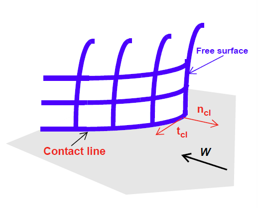
This boundary condition card is used to specify the normal velocity component on a dynamic contact line in three-dimensions. The velocity component is normal to the contact line in the plane of the web and is equal to \(V_n\). The free-surface side set should always be <bc_id1>, the primary side set, and the web side set should be <bc_id2>, the secondary side set. Usually, this boundary condition is used to model dynamic contact lines in three dimensions and is usually found in conjunction with a VELO_TANGENT_EDGE card, a VAR_CA_EDGE or CA_EDGE card as explained below.
Definitions of the input parameters are as follows:
VELO_NORMAL_EDGE |
Name of the boundary condition. |
SS |
Type of boundary condition (<bc_type>), where SS denotes side set in the EXODUS II database. |
<bc_id1> |
The boundary flag identifier, an integer associated with <bc_type> that identifies the boundary location (side set in EXODUS II) in the problem domain. This is the primary side set defining the edge and should also be associated with the capillary free surface if used in the context of a dynamic contact line. |
<bc_id2> |
The boundary flag identifier, an integer associated with <bc_type> that identifies the boundary location (side set in EXODUS II) in the problem domain. Together with <bc_id1>, this secondary side set defines the edge/curve on which the boundary condition applies as the intersection of the two side sets. In problems involving dynamic contact lines, this side set should correspond to the moving substrate. |
<float> |
\(V_n\), a parameter supplying the imposed normal velocity component. This component is taken normal to the edge curve parallel to <bc_id2>. See below for a more detailed description. |
Examples#
The following is a sample input card:
BC = VELO_NORMAL_EDGE SS 5 4 0.0
This card sets the normal-to-contact line component of the velocity to zero along the curve defined by the intersections of side set 5 and 4.
Technical Discussion#
This boundary condition imposes a point collocated constraint of the form:
where v is the fluid velocity, \(v_m\) is the mesh velocity and \(n_cl\) is the normal to the contact line in the plane of <bc_id2>. The sketch at right depicts the orientation of this latter vector. Note that the collocation points for this boundary condition only are not the nodes on the edge curve but integration points in each of the edge elements. The reason for this is historical and uninteresting from a user point of view.
This boundary condition is used almost exclusive in problems involving dynamic contact lines in three dimensions. Imposition of wetting line physics is a difficult problem in modeling situations involving dynamic contact lines. In twodimensions, the assumption is often made that the effect of any wetting line force is to locally produce a condition in which the fluid velocity at the contact line is zero in the laboratory reference frame. That is to say, that at the contact line noslip between fluid and moving substrate is not enforced and instead a zero velocity condition is imposed. In this way, the difficult-to-model wetting line forces are not included directly, but instead are included by their effect on the velocity. One might argue with this model, and many do, but as a practical approach, this has been shown to work well.
Generalizing this notion into three dimensions is the primary motivation for this boundary condition. In the case of a dynamic contact line that is a curve in three dimensions, it is not correct to simply set all velocity components to zero because that would imply that the wetting forces act equally in all three directions. It is more reasonable to say that the wetting forces can act only in a direction normal to the contact line in the plane of the substrate. Therefore, the correct generalization of the wetting line model described in the previous paragraph is to set the velocity component normal to the contact line in the plane of the substrate to zero. This is done by using the VELO_NORMAL_EDGE boundary condition with \(V_n\) set to zero. In the case of a transient problem, it is necessary to add the qualifier, “relative to the mesh motion.” This accounts for the mesh motion velocity in the constraint equation. See Baer, et.al. (2000) for a more complete discussion of this wetting line model.
Generally, a VELO_NORMAL_EDGE card must be accompanied by other boundary conditions for a correct application. Firstly, since VELO_NORMAL_EDGE forces the velocity vector to be parallel to the contact line (at least in steady state), the KINEMATIC condition on any free surface attached to the contact line will overspecify the problem at the contact line. For this reason, it is generally the case that a CA_EDGE, VAR_CA_EDGE or VAR_CA_USER (or their variants) should also be present for the contact line. These boundary conditions replace the KINEMATIC card on the mesh at the contact line.
In addition, a VELO_TANGENT_EDGE card should be present to enforce no-slip between fluid and substrate in the tangential direction. Also it should be recognized that VELO_NORMAL_EDGE will not override other Dirichlet conditions on the substrate side set. Typically, the latter are used to apply no slip between fluid and substrate. If such conditions are used over the entirety of the substrate side set, both VELO_NORMAL_EDGE and VELO_TANGENT_EDGE conditions applied at the contact will be discarded.
There are two potential solutions to this. First, the substrate region could be divided into two side sets, a narrow band of elements adjacent to the contact line and the remainder of substrate region. In the narrow band of elements, the no slip condition is replaced by a VELO_SLIP card with the substrate velocity as parameters. This allows the velocity field to relax over a finite region from the velocity imposed at the contact line to the substrate field. The second method uses only a single side set for the substrate region, but replaces the Dirichlet no slip boundary conditions with a penalized VELO_SLIP condition. That is, the slip parameter is set to a small value so that no slip is effectively enforced, but within the context of a weakly integrated condition. Since the VELO_NORMAL_EDGE and VELO_TANGENT_EDGE cards are strongly enforced on the contact lines, the VELO_SLIP card will be overridden in those locations and the velocity field will deviate appropriately from the substrate velocity.
References#
Baer, T.A., R.A. Cairncross, P.R.Schunk, R.R. Rao, and P.A. Sackinger, “A finite element method for free surface flows of incompressible fluids in three dimensions. Part II. Dynamic wetting lines.” IJNMF, 33, 405-427, (2000).
VELO_NORMAL_EDGE_INT#
BC = VELO_NORMAL_EDGE_INT SS <bc_id1> <bc_id2> <float>
Description / Usage#
(SIC-EDGE/ROTATED MOMENTUM)
This boundary condition card is used to specify the normal velocity component on a dynamic contact line in three-dimensions. The velocity component is normal to the contact line in the plane of the web and is equal to \(V_n\). The free-surface side set should always be <bc_id1>, the primary side set, and the web side set should be <bc_id2>, the secondary side set. This boundary condition is identical in function to VELO_NORMAL_EDGE. It differs only in that is applied as a strongly integrated condition along the curve defined by <bc_id1> and <bc_id2>.
Definitions of the input parameters are as follows:
VELO_NORMAL_EDGE_INT |
Name of the boundary condition. |
SS |
Type of boundary condition (<bc_type>), where SS denotes side set in the EXODUS II database. |
<bc_id1> |
The boundary flag identifier, an integer associated with <bc_type> that identifies the boundary location (side set in EXODUS II) for the primary side set in the problem domain. This side set should also be the side set associated with the capillary free surface if used in the context of a dynamic contact line. |
<bc_id2> |
The boundary flag identifier, an integer associated with <bc_type> that identifies the boundary location (side set in EXODUS II) for the secondary side set defining the edge in the problem domain. Together with <bc_id1>, this defines the curve on which the boundary condition applies as the intersection of the two side sets. In problems involving dynamic contact lines, this side set should correspond to the moving substrate. |
<float> |
\(V_n\), a parameter supplying the imposed normal velocity component value. This component is taken normal to the edge curve parallel to <bc_id2>. See below for a more detailed description. |
Examples#
The following is a sample card:
BC = VELO_NORMAL_EDGE_INT SS 5 4 0.0
This card sets the normal-to-contact line component of the velocity to zero along the curve defined by the intersections of side set 5 and 4.
Technical Discussion#
This boundary condition imposes a strongly integrated constraint of the form:
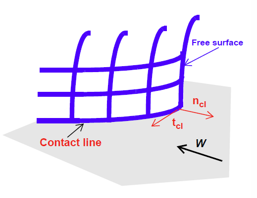
where \(\phi_i\) is the velocity trial function, v is the fluid velocity, \(v_m\) is the mesh velocity and \(n_cl\) is the normal to the contact line in the plane of the moving substrate <bc_id2>. The sketch at right depicts the orientation of this latter vector.
As noted above, this boundary condition functions nearly identically to the VELO_NORMAL_EDGE condition (except for its manner of application within Goma) and all comments appearing for the latter apply equally well for this boundary condition.
References#
No References.
VELO_TANGENT#
BC = VELO_TANGENT SS <bc_id> <integer> <float_list>
Description / Usage#
(SIC/ROTATED MOMENTUM)
This boundary condition is used to specify strongly the component of velocity tangential to the side set. An added feature is the ability to relax the condition near a point node set according to supplied length scale and slipping parameters. This has application to problems involving moving contact lines. Note that this boundary condition is applicable only to two-dimensional problems and will result in an error if it is used in a three-dimensional context.
The <float_list> has three parameters; definitions for all input parameters is as follows:
VELO_TANGENT |
Name of the boundary condition. |
SS |
Type of boundary condition (<bc_type>), where SS denotes side set in the EXODUS II database. |
<bc_id> |
The boundary flag identifier, an integer associated with <bc_type> that identifies the boundary location (side set in EXODUS II) in the problem domain. |
<integer> |
\(N_{cl}\), parameter that identifies a single-node node set that coincides with the location in the model of the moving contact line. Distances in the slipping model are computed relative to the location of this node. When the slipping model is not used, this parameter can safely be set to zero. Another toggle setting can be triggered by setting this integer to -1; with this the VELO_TANGENT condition is kept at a rolling motion dynamic contact line. (See FAQ below on rolling motion conditions.) |
<float1> |
\(v_t\), a parameter specifying the value of the tangent velocity component. The component direction is n × k where k is the z-component unit vector. |
<float2> |
\(\beta\), a parameter specifying the coefficient for slip velocity (see model below); setting \(\beta\) to zero disables the slipping model. |
<float3> |
\(\alpha\), a parameter specifying the length scale for the position dependent slip (see model below); setting \(\alpha\) to zero disables the slipping model. |
Examples#
The following is a sample input card:
BC = VELO_TANGENT SS 10 100 0.0 1.0 0.1
Technical Discussion#
Most often this boundary condition is used only to set the tangential speed on a side set because simpler Dirichlet conditions are not appropriate. An example is a sloping fully-developed inlet plane which does coincide with a coordinate axis. In this case, this boundary condition would be used to set the tangential velocity to be zero. The constraint applied at node i is as follows:
Alternatively, a dynamic contact line might be present in the problem and it is desirable that this condition be relaxed near the position of this contact line. This can be done by supplying non-zero values for \(\alpha\) and \(\beta\). In this case, the constraint that is applied at the \(i^{th}\) node on the boundary is:
in which d is the straightline distance to the node attached to <\(N_{cl}\)> and \(\dot{x}\) is the velocity vector of the mesh. It should be recognized that for steady state problems the mesh motion is by definition always zero so this constraint reverts to the previous expression.
FAQs#
Rolling Motion Conditions for high Capillary number dynamic wetting. Often times it is desirable to model a case of dynamic wetting for which the conditions result in a high capillary number. At this limit, it is well known that a contact angle specification is in fact an overspecification. Goma has always been able to model this case, except recently some changes have been made to allow for the combination of conditions at a dynamic contact line to be controlled. It should be stressed that all finite capillary number cases still work as always. This FAQ addresses the special case in which you desire to specify no-slip right up to the contact line. In most cases a VELO_SLIP card or outright setting the velocity components to zero at the moving contact line in order to impart slip will circumvent the issue taken up here.
The figure below diagrams the situation:
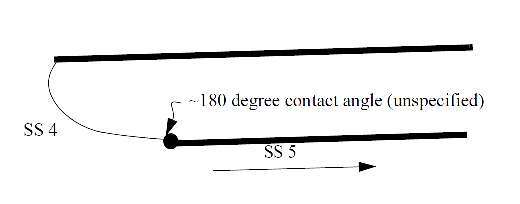
Basically the web in this example corresponds to side set 5 and the free surface to side set 4. The conditions we desire in the vicinity of the contact line are as follows:
    $web surface
BC = VELO_TANGENT SS 5   0   {web_sp}   0.0   0.0
BC = VELO_NORMAL SS 5   0.0
BC = GD_PARAB   SS 5   R_MESH2   0   MESH_POSITION1   0   0. 0. 1.
BC = GD_PARAB   SS 5   R_MESH2   0 MESH_POSITION2   0 0.   {2*roll_rad} 1.
$   upstream heel
BC = KINEMATIC SS 4 0.
BC = CAPILLARY   SS   4 {inv_cap}   0.0   0.0
Notice how there is no contact angle specified and even with the CAPILLARY card, the effect of,
VELO_NORMAL, surface tension is very small. The desired set of conditions that should be applied at the dynamic contact line are as follows:
    At node 1:
R_MOMENTUM1   gets VELO_NORMAL   from SS 5, CAPILLARY   from SS 4,
R_MOMENTUM2   gets VELO_TANGENT   from SS 5, CAPILLARY   from SS 4,
R_MESH1   gets KINEMATIC   from SS 4,
R_MESH2   gets GD_PARAB   from SS 5, GD_PARAB   from SS 5,
This clearly shows that at the contact line, which happens to be node number 1 as shown by this clip from the BCdup.txt file resulting from the run, both VELO_NORMAL and VELO_TANGENT cards are applied, which implies no-slip. This is the so-called rolling-motion case (or tank-tread on a moving surface) in which the “kinematic paradox” is no longer a paradox. That is, both the KINEMATIC condition on the free surface and the no-slip condition on the substrate can be satisfied without loss or gain of mass through the free surface (see Kistler and Scriven, 1983). In order to make sure that both the combination above is applied, a “-1” must be placed in the first integer input of the VELO_TANGENT card, vis.,
BC = VELO_TANGENT SS 5 -1 {web_sp} 0.0 0.0
This integer input slot is actually reserved for a variable slip coefficient model and is normally used to designate the nodal bc ID of the contact line. In this case of no-slip, it is not needed so we added this special control. If the following card is issued:
BC = VELO_TANGENT SS 5 0 {web_sp} 0.0 0.0
then the following combination results:
    At node 1:
R_MOMENTUM1 gets   VELO_NORMAL   from SS 5, CAPILLARY   from SS 4,
R_MOMENTUM2 gets   CAPILLARY   from SS 4,
R_MESH1 gets   KINEMATIC   from SS 4,
R_MESH2 gets   GD_PARAB   from SS 5, GD_PARAB   from SS 5,
which is desired in the case for which a contact angle and liquid slip is applied.
References#
Kistler, S. F. and Scriven, L. E. 1983. Coating Flows. In Computational Analysis of Polymer Processing. Eds. J. A. Pearson and S. M. Richardson, Applied Science Publishers, London.
VELO_TANGENT_EDGE#
BC = VELO_TANGENT_EDGE SS <bc_id1> <bc_id2> <float_list>
Description / Usage#
(PCC-EDGE/ROTATED MOMENTUM)
This boundary condition card is used to make the velocity component tangent to the contact line in the plane of the web equal to the component of web velocity (\(W_x\), \(W_y\), \(W_z\)) along the contact line. This constraint replaces the tangential component of the MOMENTUM equation along the contact line. It is used with the VELO_NORMAL_EDGE condition to impose a wetting line model onto dynamic contact lines in three-dimensions. The constraint is a rotated collocated condition.
Definitions of the input parameters are as follows:
VELO_TANGENT_EDGE |
Name of the boundary condition. |
SS |
Type of boundary condition (<bc_type>), where SS denotes side set in the EXODUS II database. |
<bc_id1> |
The boundary flag identifier, an integer associated with <bc_type> that identifies the boundary location (side set in EXODUS II) of the primary side set defining the edge geometry in the problem domain. When applied to dynamic contact lines, this side set should correspond to the free surface. |
<bc_id2> |
The boundary flag identifier, an integer associated with <bc_type> that identifies the boundary location (side set in EXODUS II) of the secondary side set defining the edge geometry in the problem domain. The boundary condition is applied to the curve defined as the intersection of this side set with the primary side set When applied to dynamic contact lines, this side set should correspond to the substrate. |
<float1> |
\(W_x\), x-component of the substrate (or web) velocity. |
<float2> |
\(W_y\), y-component of the substrate (or web) velocity. |
<float3> |
\(W_z\), z-component of the substrate (or web) velocity. |
Examples#
The following is a sample input card:
BC = VELO_TANGENT_EDGE SS 5 4 -1.0 0.0 0.0
This card imposes a tangent velocity component along the curve formed by the intersection of sidesets 5 and 4. The value of the component is the projection of the substrate velocity (-1.0, 0. ,0.) into the tangent direction. The tangent direction is along the curve itself.
Technical Discussion#
This equation imposes the following constraint as a point collocated condition at the integration points of the elements along the curve:
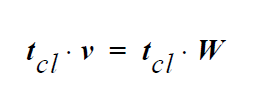
where \(t_{cl}\) is a vector tangent to the curve, v is the fluid velocity, and W is the (constant) velocity of the moving substrate. The reader is referred to the sketch appearing with the VELO_NORMAL_EDGE card for a depiction of these vectors. It is applied as a point collocated condition at the integration points of the line elements along the curve.
As noted above this boundary condition is used in concert with the VELO_NORMAL_EDGE condition to impose a model of wetting line physics along a dynamic contact line in three dimensions. The reader is referred to the discussion section of this latter boundary condition for a thorough exposition of this model. Suffice it to say that this boundary condition enforces no-slip between substrate and fluid in the tangent direction to the contact line. This is an essential part of the wetting line model because it implies that the wetting line forces related to surface tension etc. do not act tangential to the wetting line. Therefore, there is no agent in this direction which could account for departures from a strictly no-slip boundary condition.
The astute user might note that the mesh velocity doesn’t appear in this expression whereas it does in the expression for VELO_NORMAL_EDGE. In the latter expression, the normal motion of the mesh represents the wetting velocity of the contact line normal to itself. It has a physical significance and so it make senses to connect it to the fluid velocity at that point. In the case of the tangential mesh motion velocity, it cannot be attached to any obvious physical part of the wetting model. It makes no sense that the tangential motion of nodes along the contact line should induce velocity in the fluid and vice versa. As a result, mesh motion is left out of the preceding relation.
VELO_TANGENT_EDGE_INT#
BC = VELO_TANGENT_EDGE_INT SS <bc_id1> <bc_id2> <float_list>
Description / Usage#
(SIC-EDGE/ROTATED MOMENTUM)
This boundary condition card is used to make the velocity component tangent to the contact line in the plane of the web equal to the component of web velocity (\(W_x\), \(W_y\), \(W_z\)) along the contact line. It imposes the identical constraint as the VELO_TANGENT_EDGE card, but applies it as a strongly integrated condition rather than a point collocated condition.
Definitions of the input parameters are as follows:
VELO_TANGENT_EDGE_INT |
Name of the boundary condition. |
SS |
Type of boundary condition (<bc_type>), where SS denotes side set in the EXODUS II database. |
<bc_id1> |
The boundary flag identifier, an integer associated with <bc_type> that identifies the boundary location (side set in EXODUS II) of the primary side set defining the edge geometry in the problem domain. When applied to dynamic contact lines, this side set should correspond to the free surface. |
<bc_id2> |
The boundary flag identifier, an integer associated with <bc_type> that identifies the boundary location (side set in EXODUS II) of the secondary side set defining the edge geometry in the problem domain. The boundary condition is applied to the curve defined as the intersection of this side set with the primary side set When applied to dynamic contact lines, this side set should correspond to the substrate. |
<float1> |
\(W_x\), x-component of the substrate (or web) velocity. |
<float2> |
\(W_y\), y-component of the substrate (or web) velocity. |
<float3> |
\(W_z\), z-component of the substrate (or web) velocity. |
Examples#
The following is a sample input card:
BC = VELO_TANGENT_EDGE_INT SS 5 4 -1.0 0.0 0.0
This card imposes a tangent velocity component along the curve formed by the intersection of sidesets 5 and 4. The value of the component is the projection of the substrate velocity (-1.0, 0. ,0.) into the tangent direction. The tangent direction is along the curve itself.
Technical Discussion#
This equation imposes the following constraint as a point collocated condition at the integration points of the elements along the curve:
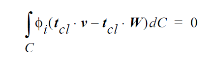
where \(t_{cl}\) is a vector tangent to the curve, v is the fluid velocity, W is the (constant) velocity of the moving substrate, \(\phi_i\) is the shape function each node along the curve C. This integral condition is imposed strongly at each node. The reader is referred to the sketch appearing with the VELO_NORMAL_EDGE card for a depiction of these vectors.
The reader is referred to the VELO_TANGENT_EDGE discussion for information about the context in which this condition is applied. Because it is applied in a different fashion than the former condition, it sometimes is the case that it will allow more flexibility in situations involving many boundary conditions applied in close proximity. There may also be situations where an integrated constraint results in better matrix conditioning that a collocated constraint.
VELO_TANGENT_3D#
BC = VELO_TANGENT_3D SS <bc_id> <float_list>
Description / Usage#
(SIC/ROTATED MOMENTUM)
This boundary condition is the three dimensional analog of the VELO_TANGENT condition. It is used to strongly set the tangential velocity component along a side set in a three-dimensional problem. It is not a completely general condition since it can set only a single tangential velocity component. It can only be applied to flat surfaces or surfaces which have only one radius of curvature such as a cylinder.
The <float_list> requires four values be specified; a description of the input parameters follows:
VELO_TANGENT_3D |
The name of the boundary condition. |
SS |
Type of boundary condition (<bc_type>), where SS denotes side set in the EXODUS II database. |
<bc_id> |
The boundary flag identifier, an integer associated with <bc_type> that identifies the boundary location (side set in EXODUS II) in the problem domain. |
<float1> |
\(v_t\), the value assigned to the tangential velocity component. |
<float2> |
\(t_x\), the x-component of a unit normal vector tangent to the surface; this vector must be tangent at all points on the surface. The direction of the imposed tangential velocity component is n × t with n the outward-pointing normal. |
<float3> |
\(t_y\), the y-component of a unit normal vector tangent to the surface; this vector must be tangent at all points on the surface. The direction of the imposed tangential velocity component is n × t with n the outwardpointing normal. |
<float4> |
\(t_z\), the z-component of a unit normal vector tangent to the surface; this vector must be tangent at all points on the surface. The direction of the imposed tangential velocity component is n × t with n the outwardpointing normal. |
Examples#
The following is an example of the card:
BC = VELO_TANGENT_3D SS 10 1.0 0.0 0.0 1.0
One could use this card to set the tangential velocity on a cylindrically shaped side set 10 provided that the cylinders axis was parallel to the z-axis. In this fashion, the tangential velocity component perpendicular to the z-axis is set to 1.0.
Technical Discussion#
The constraint applied to the velocity vector by this condition on the side set is:
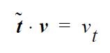
where \(\tilde{t}\) = n × t with the components of t supplied on the card. The advantages of introducing the normal vector is that it permits use of this card on curving surfaces provided the curvature occurs in only one direction and a single tangent vector exists that is perpendicular to both the surface normal and the direction of curvature. This of course implies that the tangential component can only be applied in the direction of the curvature.
Such conditions are of course met by a planar surface, but also a cylindrical surface. In the latter case, the vector t should be parallel to the axis of the cylinder. One application for this condition is in three-dimensional eccentric roll coating in which the roll speed can be set using this condition. The axis vectors of both roll coaters are supplied on the card.
VELO_SLIP#
BC = VELO_SLIP SS <bc_id> <float_list> [integer1] [float5]
Description / Usage#
(WIC/VECTOR MOMENTUM)
This boundary condition allows for slip between the fluid and a boundary using an implementation of the Navier slip relation. This relation fixes the amount of slip as a function of the applied shear stress. The scaling between stress and slip is a user parameter. This implementation also permits (in two dimensions only) variable scaling dependent upon distance from a mesh node. The latter can be used in modeling dynamic contact lines. This condition cannot currently be used on connecting surfaces.
There are four required values in <float_list> and two optional values; definitions of the input parameters are as follows:
VELO_SLIP |
Name of the boundary condition (<bc_name>). |
SS |
Type of boundary condition (<bc_type>), where SS denotes side set in the EXODUS II database. |
<bc_id> |
The boundary flag identifier, an integer associated with <bc_type> that identifies the boundary location (side set in EXODUS II) in the problem domain. |
<float1> |
\(\beta\), the slip coefficient. The inverse of \(\beta\) defines the scaling between stress and slip. Hence, for small values of \(\beta\), large shear stresses are needed for a given amount of slip, and conversely, for large values of \(\beta\), the amount of stress needed for the same degree of slip decreases (see below for a more rigorous description). |
<float2> |
\(v_{s,x}\), the x-component of surface velocity vector. This would be the x-component of the fluid velocity if a no slip condition were applied. |
<float3> |
\(v_{s,y}\), the y-component of surface velocity vector. This would be the y-component of the fluid velocity if a no slip condition were applied. |
<float4> |
\(v_{s,z}\), the z-component of surface velocity vector. This would be the z-component of the fluid velocity if a no slip condition were applied. |
[integer] |
\(N_{cl}\), a single-node node set identification number. When the variable coefficient slip relation is used, distance is measured relative to this node (see discussion below). Normally, this node set represents the location of the dynamic contact line. Note that this option is generally only used in two-dimensional simulations. |
[float5] |
\(\alpha\), the distance scale in the variable slip model (see the discussion below). Both \(N_{cl}\) and \(\alpha\) should be present to activate the variable slip model. |
Examples#
Following is a sample card without the optional parameters:
BC = VELO_SLIP SS 10 0.1 0.0 0.0 0.0
Technical Discussion#
The general form of this boundary condition is
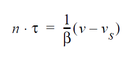
where \(\tau\) is the deviatoric portion of the fluid stress tensor, \(\beta\) is the Navier slip coefficient and \(v_s\) is the velocity of the solid surface. The velocity of the surface must be specified, as described in the Description/Usage subsection above. It is a weakly integrated vector condition, as noted above, so it will be added to each of the three momentum equation components.
This last point is important to keep in mind, especially when applying this condition to boundaries that are not parallel to any of the principle axes. It is possible under these circumstances that this condition will allow motion through a boundary curve in addition to slip tangential to it. This can be avoided by including a rotated boundary condition like VELO_NORMAL on the same sideset. This will cause the momentum equations to be rotated to normal and tangential components and also enforce no normal flow of the material. Whatever slipping that takes place will be in the tangential direction.
The variable slip coefficient model is quite simple: EQUATION, where d is the absolute distance from node \(N_{cl}\) identified on the card; the coefficients \(\beta\) and \(\alpha\) are also supplied on input. This relation is protected against overflowing as d increases. This model can be used to allow slipping to occur in a region close to the node set, but at points further removed, a no slip boundary (\(\beta\) large) is reinstated on the sideset.
VELO_SLIP_ROT#
BC = VELO_SLIP_ROT SS <bc_id> <float_list> [integer] [float5]
Description / Usage#
(WIC/VECTOR MOMENTUM)
This boundary condition is a variant of the VELO_SLIP boundary condition and serves much the same function: to allow the fluid to slip relative to a solid substrate boundary. The difference is that the assumed substrate is a rotating cylindrical surface with axis parallel to the z-direction. Also as in the VELO_SLIP case, an optional variable slip coefficient model is available that allows for slip to occur only in a region near to a mesh node. This boundary condition is applicable generally only to two-dimensional problems or very specialized three dimensional problems.
The <float_list> has four values and there are two optional values; definitions of the input parameters are as follows:
VELO_SLIP_ROT |
Name of the boundary condition. |
SS |
Type of boundary condition (<bc_type>), where SS denotes side set in the EXODUS II database. |
<bc_id> |
The boundary flag identifier, an integer associated with <bc_type> that identifies the boundary location (side set in EXODUS II) in the problem domain. |
<float1> |
\(\beta\) the slip coefficient. The inverse of \(\beta\) defines the scaling between stress and slip. Hence, for small values of \(\beta\), large shear stresses are needed for a given amount of slip, and conversely, for large values of \(\beta\), the amount of stress needed for the same degree of slip decreases (see below for a more rigorous description). |
<float2> |
\(\omega\), rotation rate of the cylindrical substrate surface in radians/T. Positive values for this parameter correspond to rotation in the clockwise direction. |
<float3> |
\(x_c\), the x-position of rotation axis. |
<float4> |
\(y_c\), the y-position of rotation axis. |
[integer] |
\(N_{cl}\), a single-node node set identification number. When variable coefficient slip relation is used, distance is measured relative to this node (see discussion below). For problems involving dynamic contact lines, this nodeset coincides with the location of the contact line. |
[float5] |
\(\alpha\), the distance scale in the variable slip model (see the discussion below). Both \(N_{cl}\) and \(\alpha\) should be present to activate the variable slip model. |
Examples#
The following is a sample card without the optional parameters:
BC = VELO_SLIP_ROT SS 10 0.1 3.14 0.0 1.0
This condition specifies a moderate amount of slip (0.1) on a cylindrical surface rotating at 3.14 rad/sec around the point (0.0,1.0).
Technical Discussion#
The comments that appear in the Technical Discussion section of the VELO_SLIP card apply equally well here. In particular, the discussion of the variable slip coefficient model applies here as well. The only significant difference is that the velocity of the substrate is not a fixed vector; instead, it is tangent to the cylindrical substrate with a magnitude consistent with the radius of the cylinder and the rotation rate.
References#
No References.
VELO_SLIP_FILL#
BC = VELO_SLIP_FILL SS <bc_id> <float_list>
Description / Usage#
(WIC/VECTOR MOMENTUM)
This boundary condition is applied only in problems involving embedded interface tracking, that is, level set or volume of fluid. As in the case of the VELO_SLIP card, it allows for slip to occur between fluid and solid substrate, but in this case slipping is allowed only in a narrow region around the location of the interface where it intercepts the solid boundary. Elsewhere, this boundary condition enforces a no-slip condition between fluid and substrate.
When using the level set tracking, slip is allowed only near the intersection of the zero level set contour and the substrate boundary, and then only in a region twice the level set length scale wide centered on the zero level set. When using volume of fluid, the criterion for slipping is that the absolute value of the color function should be less than 0.25.
This boundary condition is most often used in conjunction with the FILL_CA boundary condition. The latter applies forces to contact lines in order to simulate wetting line motion. These forces are applied in a weak sense to the same regions near the interface so it is necessary to use VELO_SLIP_FILL with a large slipping coefficient so that effectively no-slip is relaxed completely near the interface.
Definitions of the input parameters are as follows:
VELO_SLIP_FILL |
Name of the boundary condition. |
SS |
Type of boundary condition (<bc_type>), where SS denotes side set in the EXODUS II database. |
<bc_id> |
The boundary flag identifier, an integer associated with <bc_type> that identifies the boundary location (side set in EXODUS II) in the problem domain. |
<float1> |
\(\beta\), the slip coefficient. The inverse of \(\beta\) defines the scaling between stress and slip. The parameter supplied on the input deck is used only in the region define above. Elsewhere, the slip coefficient is uniformly set to \(10^{-6}\). |
<float2> |
\(v_{s,x}\), the x-component of surface velocity vector. This would be the x-component of the fluid velocity if a noslip condition were applied. |
<float3> |
\(v{s,y}\), the y-component of surface velocity vector. This would be the y-component of the fluid velocity if a noslip condition were applied. |
<float4> |
\(v{s,z}\), the z-component of surface velocity vector. This would be the z-component of the fluid velocity if a noslip condition were applied. |
Examples#
Following is a sample card without the optional parameters:
BC = VELO_SLIP SS 10 100000.0 0.0 0.0 0.0
The large value of slip coefficient ensures nearly perfect slip in the region around the interface.
Technical Discussion#
See the documentation under VELO_SLIP boundary condition for a description of the nature of this boundary condition.
An important caveat when using this boundary condition to relax no-slip in the vicinity of the interface is that it relaxes all constraints on the velocities in the region. This includes the constraint to keep fluid from passing through the substrate boundary. For this region, it is usually also necessary to use a impenetrability condition, VELO_NORMAL for example, in conjunction with this boundary condition for appropriate results.
References#
No References.
VELO_SLIP_ELECTROKINETIC#
BC = VELO_SLIP_ELECTROKINETIC SS <bc_id> <float1> <float2>
Description / Usage#
(SIC/ROTATED MOMENTUM)
This boundary condition allows for slip between the fluid and a solid boundary due to electrokinetic effects on the charged solid wall. The user provides the following parameters: zeta potential at the wall and permittivity of the fluid.
VELO_SLIP_ELECTROKINETIC |
Name of the boundary condition (<bc_name>). |
SS |
Type of boundary condition (<bc_type>), where SS denotes side set in the EXODUS II database. |
<bc_id> |
The boundary flag identifier, an integer associated with <bc_type> that identifies the boundary location (side set in EXODUS II) in the problem domain. |
<float1> |
\(\varepsilon\), absolute permittivity of the fluid. |
<float2> |
\(\zeta\), the surface potential of solid boundary. It is referred to as the zeta potential. |
Examples#
Following is a sample card:
BC = VELO_SLIP_ELECTROKINETIC SS 10 1.e-5 1.e-2
Technical Discussion#
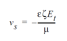
The general form of this boundary condition is
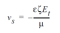
where \(\varepsilon\) is the absolute permittivity of the medium, \(\zeta\) is the zeta potential, \(E_t\) is the electric field tangent to the solid surface, and \(v_s\) is the slip velocity.
VELO_SLIP_ELECTROKINETIC3D#
BC = VELO_SLIP_ELECTROKINETIC3D SS <bc_id> [floatlist]
Description / Usage#
(SIC/ROTATED MOMENTUM)
This is a 3D generalization of the VELO_SLIP_ELECTROKINETIC boundary condition. It is similar to VELO_TANGENT_3D except the slip velocity is calculated based on Helmholtz-Smulkowski relation. This boundary condition allows for slip between the fluid and a solid boundary due to electrokinetic effects on the charged solid wall. The user provides the following parameters: zeta potential at the wall, permittivity of the fluid and.
VELO_SLIP_ELECTROKINETIC3D |
Name of the boundary condition (<bc_name>). |
SS |
Type of boundary condition (<bc_type>), where SS denotes side set in the EXODUS II database. |
<bc_id> |
The boundary flag identifier, an integer associated with <bc_type> that identifies the boundary location (side set in EXODUS II) in the problem domain. |
<float1> |
\(\varepsilon\), absolute permittivity of the fluid. |
<float2> |
\(\zeta\), the surface potential of solid boundary. It is referred to as the zeta potential. |
<float3> |
\(t_x\), the x-component of a unit normal vector tangent to the surface; this vector must be tangent at all points on the surface. The direction of the imposed tangential velocity component is n × t with n the outwardpointing normal. |
<float4> |
\(t_y\), the y-component of a unit normal vector tangent to the surface; this vector must be tangent at all points on the surface. The direction of the imposed tangential velocity component is n × t with n the outwardpointing normal. |
<float5> |
\(t_z\), the z-component of a unit normal vector tangent to the surface; this vector must be tangent at all points on the surface. The direction of the imposed tangential velocity component is n × t with n the outwardpointing normal. |
Examples#
Following is a sample card:
BC = VELO_SLIP_ELECTROKINETIC3D SS 10 1.e-5 1.e-2 0. 0. 1.
Technical Discussion#
The general form of this boundary condition is
where \(\varepsilon\) is the absolute permittivity of the medium, \(\zeta\) is the zeta potential, \(E_t\) is the electric field tangent to the solid surface, and \(v_s\) is the slip velocity.
VELO_TANGENT_SOLID#
BC = VELO_TANGENT_SOLID SS <bc_id> <integer1> <integer2>
Description / Usage#
(SIC/ROTATED MOMENTUM)
This boundary condition sets the tangential fluid velocity component at a fluid/solid interface to the tangential velocity component of the solid material. The latter includes any motion of the stress-free state. This boundary condition is applicable only to twodimensional problems and is normally used in conjunction with the Total Arbitrary Lagrangian/Eulerian algorithm in Goma (See GT-005.3).
Definitions of the input parameters are as follows:
VELO_TANGENT_SOLID |
The name of the boundary condition. |
SS |
Type of boundary condition (<bc_type>), where SS denotes side set in the EXODUS II database. |
<bc_id> |
The boundary flag identifier, an integer associated with <bc_type> that identifies the boundary location (side set in EXODUS II) in the problem domain. |
<integer1> |
The element block id defining the solid phase adjacent to <bc_id>. |
<integer2> |
The element block id defining the liquid phase adjacent to <bc_id>. |
Examples#
The following is an example of this card
BC = VELO_TANGENT_SOLID SS 10 2 1
In this case, sideset 10 is an internal sideset between two separate materials, the solid material in element block 2 and the liquid material in element block 1.
Technical Discussion#
The boundary condition being applied is the strong integrated condition:
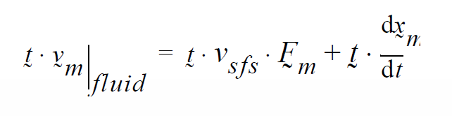
where \(v_m\) is the fluid velocity, \(v_{sfs}\) is the velocity of the solid material stress-free-state (usually solid-body translation, or rotation..see Advected Langragian Velocity card) including the motion of the deformed coordinates, and t is the vector tangent to the side set. \(F_m\) is the deformation gradient tensor and the time derivative term is the motion of the deformed state tangential to the surface in question.
This condition is advocated for use with the TALE algorithm (see GT-005.3).
VELO_SLIP_SOLID#
BC = VELO_SLIP_SOLID SS <bc_id> <integer_list> <float1> [integer3, float2]
Description / Usage#
(WIC/ROTATED MOMENTUM)
This boundary condition is similar in function to the VELO_SLIP condition in that it permits a tangential velocity in a fluid phase to be proportional to the shear stress at the boundary. This boundary condition allows for this type of slip to occur at the interface between a fluid material and a LAGRANGIAN or TALE solid material. The velocity of the solid substrate is obtained automatically from the motion of the solid material, including advection of the stress-free state. As in the case of the VELO_SLIP condition, this condition also permits the user to vary the slip coefficient depending upon the distance from a specified point in the mesh. The variable slip model can only be used in two-dimensional problems.
The <integer_list> has two values; the definitions of the input parameters and their significance in the boundary condition parameterization is described below:
VELO_SLIP_SOLID |
Name of the boundary condition. |
SS |
Type of boundary condition (<bc_type>), where SS denotes side set in the EXODUS II database. |
<bc_id> |
The boundary flag identifier, an integer associated with <bc_type> that identifies the boundary location (side set in EXODUS II) in the problem domain. This should be an internal sideset defined at the interface between solid and liquid material blocks. |
<integer1> |
The element block id defining the solid material phase. |
<integer2> |
The element block id defining the liquid material phase. |
<float1> |
\(\beta\), the slip coefficient. The inverse of \(\beta\) defines the scaling between stress and slip. Hence, for small values of \(\beta\), large shear stresses are needed for a given amount of slip, and conversely, for large values of \(\beta\), the amount of stress needed for the same degree of slip decreases (see below for a more rigorous description). |
[integer3] |
\(N_{cl}\), a single-node node set identification number. When the variable coefficient slip relation is used, distance is measured relative to this node (see discussion below). Normally, this node set represents the location of the dynamic contact line. Note that this option is generally only used in two-dimensional simulations. |
[float2] |
\(\alpha\), the distance scale in the variable slip model (see the discussion below). Both \(N_{cl}\) and \(\alpha\) should be present to activate the variable slip model. |
Examples#
The following is a sample card:
BC = VELO_SLIP_SOLID SS 20 2 1 0.001 0.0 4 0.01
This boundary condition sets the slip coefficient between solid material 2 and liquid material 1 to be 0.001 except in the vicinity of the nodeset 4 (a single node) where the variable model is used.
Technical Discussion#
The general form of this boundary condition is
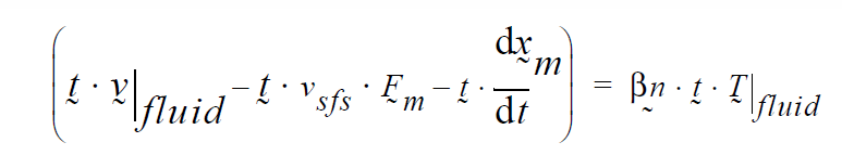
where \(\tau\) is the deviatoric portion of the fluid stress tensor, \(\beta\) is the Navier slip coefficient and \(v_{sfs}\) is the velocity of the solid surface stress-free state, with \(F_m\) the deformation gradient tensor; this motion includes any rigid solid body motion and any superimposed deformation velocity.
It is worthwhile noting that, unlike the VELO_SLIP condition, this condition is actually a rotated condition. It is applied to the tangential component of the rotated momentum equations weakly. This means that the normal component of the momentum equation is not affected by this boundary condition. Normally, some sort of no-penetration condition must accompany this boundary condition for this reason.
The reader is referred to the documentation of the variable slip coefficient model to apply slip near contact lines under the VELO_SLIP boundary condition.
VELO_SLIP_POWER#
BC = VELO_SLIP_POWER SS <bc_id> <float_list>
Description / Usage#
(WIC/VECTOR MOMENTUM)**
This boundary condition allows for slip between the fluid and a boundary using an implementation of the Navier slip relation. This relation fixes the amount of slip as a function of the applied shear stress. The scaling between stress and slip is a user parameter.
The slip velocity is in the tangential direction \(t \cdot v_{slip}\) and is raised to a power (user param m)
There is an optional tangent vector to be input to the BC, the BC expects this vector to be a unit tangent vector.
There are five required values in <float_list> and three optional values; definitions of the input parameters are as follows:
- VELO_SLIP_POWER
Name of the boundary condition (<bc_name>).
- SS
Type of boundary condition (<bc_type>), where SS denotes side set in the EXODUS II database.
- <bc_id>
The boundary flag identifier, an integer associated with <bc_type> that identifies the boundary location (side set in EXODUS II) in the problem domain.
- <float1>
\(\beta\), the slip coefficient. The inverse of \(\beta\) defines the scaling between stress and slip.
- <float2>
\(v_{s,x}\), the x-component of surface velocity vector. This would be the x-component of the fluid velocity if a no slip condition were applied.
- <float3>
\(v_{s,y}\), the y-component of surface velocity vector. This would be the y-component of the fluid velocity if a no slip condition were applied.
- <float4>
\(v_{s,z}\), the z-component of surface velocity vector. This would be the z-component of the fluid velocity if a no slip condition were applied.
- <float5>
\(m\), the power to raise the slip velocity to
- [float6]
\(t_x\), x-component of tangent vector
- [float7]
\(t_y\), y-component of tangent vector
- [float8]
\(t_z\), z-component of tangent vector
Examples#
Following is a sample card without the optional parameters:
BC = VELO_SLIP_POWER SS 10 0.1 0.0 0.0 0.0 2.0
Technical Discussion#
Boundary condition of the form:
Theory#
No Theory.
FAQs#
No FAQs.
References#
VELO_SLIP_POWER_CARD#
BC = VELO_SLIP_POWER_CARD SS <bc_id> <float_list>
Description / Usage#
(WIC/VECTOR MOMENTUM)**
This boundary condition allows for slip between the fluid and a boundary using an implementation of the Navier slip relation. This relation fixes the amount of slip as a function of the applied shear stress. The scaling between stress and slip is a user parameter.
The slip velocity is a vector and is raised to a power component-wise.
There are five required values in <float_list> and three optional values; definitions of the input parameters are as follows:
- VELO_SLIP_POWER_CARD
Name of the boundary condition (<bc_name>).
- SS
Type of boundary condition (<bc_type>), where SS denotes side set in the EXODUS II database.
- <bc_id>
The boundary flag identifier, an integer associated with <bc_type> that identifies the boundary location (side set in EXODUS II) in the problem domain.
- <float1>
\(\beta\), the slip coefficient. The inverse of \(\beta\) defines the scaling between stress and slip.
- <float2>
\(v_{s,x}\), the x-component of surface velocity vector. This would be the x-component of the fluid velocity if a no slip condition were applied.
- <float3>
\(v_{s,y}\), the y-component of surface velocity vector. This would be the y-component of the fluid velocity if a no slip condition were applied.
- <float4>
\(v_{s,z}\), the z-component of surface velocity vector. This would be the z-component of the fluid velocity if a no slip condition were applied.
- <float5>
\(m\), the power to raise the slip velocity to
Examples#
Following is a sample card without the optional parameters:
BC = VELO_SLIP_POWER_CARD SS 10 0.1 0.0 0.0 0.0 2.0
Technical Discussion#
Boundary condition of the form:
Theory#
No Theory.
FAQs#
No FAQs.
References#
DISCONTINUOUS_VELO#
BC = DISCONTINUOUS_VELO SS <bc_id> <char_string> <integer1> <integer2>
Description / Usage#
(SIC/MOMENTUM)
This boundary condition card, used to set the normal component of mass averaged velocity at an interface, specifies that the net flux of the last component in a nondilute mixture across an internal interface, is equal to zero. The condition only applies to interphase mass, heat, and momentum transfer problems applied to nondilute material phases with discontinuous (or multivalued) variables at an interface, and it must be invoked on fields that employ the Q1_D or Q2_D interpolation functions to “tie” together or constrain the extra degrees of freedom at the interface in question.
Definitions of the input parameters are as follows:
DISCONTINOUS_VELO |
Name of the boundary condition (<bc_name>). |
SS |
Type of boundary condition (<bc_type>), where SS denotes side set in the EXODUS II database. |
<bc_id> |
The boundary flag identifier, an integer associated with <bc_type> that identifies the boundary location (side set in EXODUS II) in the problem domain. |
<char_string> |
A character string identifiying the condition to be applied on the liquid phase relative to the gas phase.
Note, this parameter replaces the boundary condition EVAPORATION_VELO. |
<integer1> |
Element block id of liquid or high density phase. |
<integer2> |
Element block id of gas or low density phase. |
Examples#
Following is a sample input card that applies this BC on the block 1 side of side set 7, the liquid side; the block 2 side is the gas side.
BC = DISCONTINUOUS_VELO SS 7 EVAPORATION 1 2
Technical Discussion#
The DISCONTINUOUS_VELO boundary condition applies the following equation:
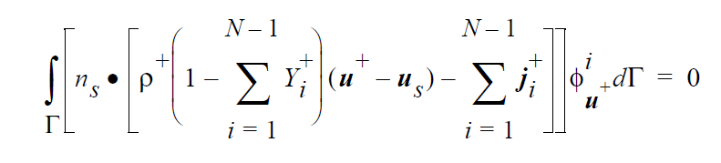
It specifies the diffusive flux of the last species in the mechanism, i.e., the one for which no explicit continuity equation exists, to be equal to zero. This is done via a strong integral condition applied to one side of the interface, the “+” side of the interface. This boundary condition, combined with the KINEMATIC_SPECIES and KINEMATIC_DISC boundary conditions, implies that the diffusive flux of the last species on both sides of the boundary is equal to zero.
The DISCONTINUOUS_VELO boundary condition requires an evaluation of the derivative of the species mass fraction at the interface. Thus, the mesh convergence properties of the algorithm are reduced to O( h ). Also, discretization error must interfere with the total mass balance across a phase, since the expression for \(j_i^+\) is substituted for in some places, the YFLUX_SPECIES boundary condition, but used in the DISCONTINUOUS_VELO boundary condition.
HYDROSTATIC_SYMM#
BC = HYDROSTATIC_SYMM
Description / Usage#
(WIC/VECTOR MOMENTUM)
No longer supported in GOMA. Do not use.
Examples#
No Example.
Technical Discussion#
No Discussion.
References#
No References.
FLOW_PRESSURE#
BC = FLOW_PRESSURE SS <bc_id> <float>
Description / Usage#
(WIC/VECTOR MOMENTUM)
This boundary condition card is used to set a constant value of pressure on a boundary. Most often this condition is used to set an upstream or downstream pressure over a fully-developed inflow/outflow boundary.
Definitions of the input parameters are as follows:
FLOW_PRESSURE |
Boundary condition name. |
SS |
Type of boundary condition (<bc_type>), where SS denotes side set in the EXODUS II database. |
<bc_id> |
The boundary flag identifier, an integer associated with <bc_type> that identifies the boundary location (side set in EXODUS II) in the problem domain. |
<float> |
\(P_{ex}\), the applied pressure. Positive values imply compressive forces on the fluid, negative values imply tensile forces. |
Examples#
The following sample input card will impose a constant compressive pressure force on the boundary defined by sideset 23:
BC = FLOW_PRESSURE SS 23 5.0
Technical Discussion#
The actual boundary condition that is applied to the fluid is given as follows:
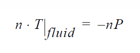
where n is the outward normal vector to the boundary, T is the total fluid stress tensor, and P is the applied pressure equal to <float1> above. From this the user should be able to deduce the appropriate sign for his/her pressure value.
This boundary condition is a weak integrated condition implying that it is added to all three components of the fluid momentum equation prior to rotation of equations or application of strongly enforced conditions or Dirichlet conditions.
The astute user who is also well-versed in finite element formulations and terminology will recognize that this boundary condition is providing a value for the boundary condition term that appears after application of the divergence theorem to the weighted fluid momentum residual equations. Hence, imposing a value of zero for <float1> is exactly equivalent to saying nothing at all about the fluid velocity at a boundary.
This boundary condition is found predominantly in two applications. First, setting the external pressure imposed on a free surface, and second, providing the driving force for flow by being imposed on an inflow or outflow fully-developed boundary. In this latter role, the usual procedure is to apply the FLOW_PRESSURE condition while strongly enforcing a zero condition on the velocity components transverse to the boundary. For boundaries parallel to one of the principle coordinate directions, Dirichlet conditions can be used to set these transverse components. For other inflow or outflow boundaries, it is suggested that the VELO_TANGENT and VELO_TANGENT_3D cards be employed instead.
This boundary condition is very useful when working with non-Newtonian models where the inlet velocity field is apt to be complicated and hard to determine a priori. By imposing a pressure at the inflow with this card, the non-Newtonian inlet velocity profile will be determined implicitly. Augmenting conditions can then be used to couple the imposed pressure to the average flow rate over the boundary for an even more advanced capability.
FLOW_STRESSNOBC#
BC = FLOW_STRESSNOBC SS <bc_id> <float> [integer]
Description / Usage#
(WIC/VECTOR MOMENTUM)
This boundary condition card applies the free outflow boundary condition developed by Papanastasiou, et.al. (1992) on the fluid momentum with the option of setting the pressure level. It is appropriate only for outflow boundaries where it is inappropriate to use natural boundary conditions or FLOW_PRESSURE-class boundary conditions. It is only supported for generalized Newtonian fluid constitutive equations.
Definitions of the input parameters are as follows:
FLOW_STRESSNOBC |
Name of the boundary condition. |
SS |
Type of boundary condition (<bc_type>), where SS denotes side set in the EXODUS II database. |
<bc_id> |
The boundary flag identifier, an integer associated with <bc_type> that identifies the boundary location (side set in EXODUS II) in the problem domain. |
<float> |
\(P_{applied}\), the applied pressure. |
[integer] |
An optional parameter.
|
Examples#
Following is a sample card:
BC = FLOW_STRESSNOBC SS 10 1.0 -1
Here the boundary condition is applied to sideset 10 with a constant pressure of 1.0 required.
Technical Discussion#
The finite element formulation of the fluid momentum equations generates boundary integrals of the form:
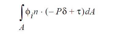
where P is the isotropic pressure and \(\tau\) the viscous stress. Often this boundary term is left off entirely on a particular boundary with the result that a zero normal force is applied implicitly. These are referred to as imposing a “natural” boundary conditions. Alternatively, this integral might be included but with the integrand replaced by an known value of force. This is the concept behind the FLOW_PRESSURE and FLOW_HYDROSTATIC boundary conditions.
However, both types of boundary conditions imply that something is known about the stress and, by association, the velocity field on the boundary. It is often the case that outflow boundaries are present where it is difficult to provide this information. A prime example is the outflow of a fluid jet accelerating downward due to gravity. In this case, the downward velocity field is still developing at this boundary so it is problematic to specify a stress value. Other examples include imposing conditions at a “truncated” outflow where the exiting fluid is still developing.
The FLOW_STRESSNOBC seeks to remedy this problem. Formulationally, the boundary term as written above is included as just another term dependent upon solution degrees of freedom. This permits the pressure and velocity gradients on the boundary to float as needed so that one does not need to say anything about the stress or pressure on the boundary.
Now strictly speaking, the ellipticity of the viscous flow equations suggests that this operation should result in an ill-posed problems. Elliptic equations by their very nature require that something be said about every boundary in the problem. However, in the case of outflow boundaries it appears that this restriction can be relaxed in certain circumstances with good results. Papanastasiou, et.al., (1997), Renary (1997), Griffiths (1997) and Sani and Gresho (1994) discuss this.
The boundary condition does permit that the pressure value be fixed while the viscous stress is allowed to float. This is done by setting the optional parameter to -1 and supplying the pressure value as \(P_{applied}\). When this is done depends upon circumstance. Note that this is distinctly different from setting a normal stress component using FLOW_PRESSURE.
As noted above, this boundary condition is currently implemented only for generalized Newtonian fluid models. Polymeric fluid models will not work with it.
References#
Griffiths, D.F., “The ‘no boundary condition’ outflow boundary condition,” IJNMF, 24, 393-411, (1997)
Papanastasiou, T. C., N. Malamataris, and K. Ellwood, “A New Outflow Boundary Condition”, IJNMF, 14, 587-608, (1992).
Renardy, M., “Imposing ‘NO’ boundary conditions at outflow: Why does this work?” IJNMF, 24, 413-417, (1997).
Sani, R.L., and P.M. Gresho, “Resume and remarks on the open boundary condition minisymposium,” IJNMF, 18, 983-1008, (1994).
FLOW_GRADV#
BC = FLOW_GRADV SS <bc_id> <float> [integer]
Description / Usage#
(WIC/VECTOR MOMENTUM)
This boundary condition card stipulates a vanishing normal velocity gradient on a boundary with the option of setting the pressure level.
Definitions of the input parameters are as follows:
FLOW_GRADV |
Name of the boundary condition. |
|
SS |
Type of boundary condition (<bc_type>), where SS denotes side set in the EXODUS II database. |
|
<bc_id> |
The boundary flag identifier, an integer associated with <bc_type> that identifies the boundary location (side set in EXODUS II) in the problem domain. |
|
<float> |
\(P_{applied}\), the applied pressure. |
|
[integer] |
An optional parameter. |
|
blank/-1 |
the pressure in the normal stress is replaced by \(P_{applied}\). |
|
≠ –1 |
|
|
Examples#
The sample input card:
BC = FLOW_GRADV SS 15 0.0
sets the gradient of velocity normal to sideset 15 to zero. A pressure value of zero is used in the boundary condition.
BC = FLOW_GRADV SS 15 0.0 1.0
In the preceding example, the pressure value used is obtained from the solution itself.
Technical Discussion#
This boundary condition is related in form and formulation to the FLOW_STRESSNOBC boundary condition in that it includes terms for the boundary integrals that appear in the momentum equation after application of integration by parts and the divergence theorem. In this boundary condition, the following integral is included with the momentum equation:
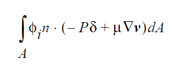
where \(\mu\) is the viscosity of a Newtonian or generalized Newtonian fluid. As in the case of the FLOW_STRESSNOBC condition the preceding integral appears as a function of pressure and velocity unknowns as any other term.
The pressure term in the preceding may be replaced by a fixed, imposed pressure value. This is done by setting the optional input integer to -1 and providing the imposed value in \(P_{applied}\) ; otherwise, the value set in \(P_{applied}\) is ignored.
FLOW_GRADV_T#
BC = FLOW_GRADV_T SS <bc_id> <float> [integer]
Description / Usage#
(WIC/VECTOR MOMENTUM)
This boundary condition card stipulates a vanishing normal velocity gradient on a boundary with the option of setting the pressure level.
Definitions of the input parameters are as follows:
- FLOW_GRADV_T
Name of the boundary condition.
- SS
Type of boundary condition (<bc_type>), where SS denotes side set in the EXODUS II database.
- <bc_id>
The boundary flag identifier, an integer associated with <bc_type> that identifies the boundary location (side set in EXODUS II) in the problem domain.
- <float>
\(P_{applied}\), the applied pressure.
- [integer]
An optional parameter.
blank/-1 the pressure in the normal stress is replaced by \(P_{applied}\).
≠ –1 the pressure in the solution vector is retained in the normal stress.
Examples#
The sample input card:
BC = FLOW_GRADV_T SS 15 0.0
sets the transpose of gradient of velocity normal to sideset 15 to zero. A pressure value of zero is used in the boundary condition.
BC = FLOW_GRADV_T SS 15 0.0 1.0
In the preceding example, the pressure value used is obtained from the solution itself.
Technical Discussion#
This boundary condition is related in form and formulation to the FLOW_STRESSNOBC boundary condition in that it includes terms for the boundary integrals that appear in the momentum equation after application of integration by parts and the divergence theorem. In this boundary condition, the following integral is included with the momentum equation (for Newtonian):
where \(\mu\) is the viscosity of a Newtonian or generalized Newtonian fluid. As in the case of the FLOW_STRESSNOBC condition the preceding integral appears as a function of pressure and velocity unknowns as any other term.
This imposes a natural BC of \(n\cdot\nabla v = 0\)
The pressure term in the preceding may be replaced by a fixed, imposed pressure value. This is done by setting the optional input integer to -1 and providing the imposed value in \(P_{applied}\) ; otherwise, the value set in \(P_{applied}\) is ignored.
Modifications are done to work for Viscoelastic flow with DEVSS-G stabilization
FLOW_PRESS_USER#
BC = FLOW_PRESS_USER
Description / Usage#
(WIC/VECTOR MOMENTUM)
This boundary condition has been deprecated in favor of the PRESSURE_USER boundary condition; use the latter instead.
Examples#
No Examples.
Technical Discussion#
No Discussion.
References#
No References.
FLOW_HYDROSTATIC#
BC = FLOW_HYDROSTATIC SS <bc_id> <float_list>
Description / Usage#
(WIC/VECTOR MOMENTUM)
This boundary condition allows the user to impose a pressure force that varies linearly with position over the boundary. It functions in much the same manner as the FLOW_PRESSURE boundary condition except that more variability is allowed in the imposed pressure. As the name implies, this boundary condition is most often used to impose hydrostatic pressure profiles in problems in which gravitational forces play a role.
The <float_list> has four values to be specified; definitions of the input parameters are as follows:
FLOW_HYDROSTATIC |
Boundary condition name. |
SS |
Type of boundary condition (<bc_type>), where SS denotes side set in the EXODUS II database. |
<bc_id> |
The boundary flag identifier, an integer associated with <bc_type> that identifies the boundary location (side set in EXODUS II) in the problem domain. |
<float1> |
\(\delta P_x\), the pressure variation in x-direction. |
<float2> |
\(\delta P_y\), the pressure variation in y-direction. |
<float3> |
\(\delta P_z\), the pressure variation in z-direction. |
<float4> |
\(P_0\), the pressure value at the coordinate point (0,0,0). This serves as a means of establishing a datum and it is not required that (0,0,0) lie on the sideset. |
Examples#
Following is a sample card:
BC = FLOW_HYDROSTATIC SS 15 0.0 0.0 -1.5 10.0
This card will impose a pressure profile on side set 15 so that the pressure decreases by 1.5 as the z coordinate increases by one unit. At the point, (0,0,0) the pressure imposed is 10.0. Note that (0,0,0) does not necessarily have to be on side set 15.
Technical Discussion#
The mathematical form of the boundary condition imposed by this card is as follows:
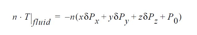
where n is the outward normal vector to the boundary, T is the total fluid stress tensor, and x, y, z are the global coordinate positions.
Like the FLOW_PRESSURE conditions, this is a weakly integrated condition and the comments appearing with that card apply equally well here.
Most often this boundary condition is used in problems in which gravity is present. Under these circumstances, the pressure profile across a fully-developed flow inlet is not constant but varies according to hydrostatic head. Hence, the FLOW_PRESSURE condition cannot be used to provide the inlet pressure. Instead, this card is used with the variation in the pressure being imposed according to the direction of gravity. Thus, some if not all of \(\delta P_x\), \(\delta P_y\), or \(\delta P_z\) will be functions of gravity and the fluid density.
It is true that this variation could be determined automatically by Goma from its known values for density and gravitational direction. But for a variety of reasons, this may not always be the best option. Instead, the user is allowed to vary the pressure on a boundary independently of the density and gravitational forces set elsewhere in the material file. If consistency is important in the problem at hand, then the user is cautioned to be consistent.
The input parameter \(P_0\) as noted above serves as a datum to the relationship. In theory, it is the pressure value that would be computed at the point (0,0,0), but in reality it is chosen to impose a known pressure at some point in the domain.
References#
No References.
FLOWRATE#
BC = FLOWRATE SS <bc_id> <float> <float | char_string>
Description / Usage#
(WIC/VECTOR MOMENTUM)
This boundary condition allows the user to specify a single value for the volumetric flowrate of material across an inflow (or outflow) boundary. The pressure and velocity fields on this boundary are then computed implicitly by Goma.
Definitions of the input parameters are as follows:
FLOWRATE |
Boundary condition name. |
|
SS |
Type of boundary condition (<bc_type>), where SS denotes side set in the EXODUS II database. |
|
<bc_id> |
The boundary flag identifier, an integer associated with <bc_type> that identifies the boundary location (side set in EXODUS II) in the problem domain. |
|
<float> |
flowrate, a parameter fixing the value of volumetric flowrate across this boundary. For two-dimensional CARTESIAN simulations, this value should be per unit distance in the out-of-plane coordinate. For CYLINDRICAL and SWIRLING coordinate systems, this flowrate value should include integration in the azimuthal direction. |
|
<float|char_string> |
This parameter can either be a <float> or a <char_string>. |
|
float |
\(P_{guess}\), an initial guess for the pressure on the inlet |
|
char_string |
read, indicating that the initial guess for the pressure file should be read from the ASCII file identified on the GUESS file card. |
|
Examples#
Specifying the average velocity on the inlet to a tube of radius 1.0:
BC = FLOWRATE SS 10 3.1415 10.0
Since the radius is 1.0, the area of the surface is 3.1415 so the volumetric flowrate must be specified as shown. An initial pressure guess of 10.0 is also supplied. Note this does not specify the pressure on the boundary as the final value will generally be different than specified here.
Continuing in the flowrate by reading the last pressure value from GUESS file:
BC = FLOWRATE SS 10 3.2 read
Technical Discussion#
The requirement that is imposed by this boundary condition is the following integral:
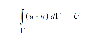
where U is the flowrate value supplied on the card. It is imposed by the addition of a Lagrange multiplier unknown on the boundary in question which will be determined as a part of the solution process. For Newtonian and generalized Newtonian models, the value of the multiplier is the inverse of the pressure value on the boundary. Thus, a boundary condition nearly identical to a FLOW_PRESSURE condition is applied to the sideset, but it takes as its pressure the value of the inverse of the Lagrange multiplier unknown as it is computed.
The augmenting condition capability in Goma is used to impose the above integral. When the boundary condition is invoked, an augmenting condition of the appropriate type is automatically created. Its associated degree of freedom is the Lagrange multiplier. During the iteration sequence, the user will see updates and residuals for this augmenting condition.
Originally, the initial guessed value for the pressure over the side set is read from the float value specified on this card, or from the GUESS file (if the parameter read is specified on this card). However, it can also be read from an EXODUS II database file. This is the same file the rest of the solution vector is read from if the problem is being restarted from a previous computation. If a value for the augmenting condition is present in this EXODUS II file, it will be read in. This value will override the float value specified on this card. The initial guess may still be read from the ASCII GUESS file by specifying read on the Initial Guess card and on the Augmenting Conditions Initial Guess card.
References#
No References.
PRESSURE_USER#
BC = PRESSURE_USER SS <bc_id> <float_list>
Description / Usage#
(WIC/VECTOR MOMENTUM)
This boundary condition allows the user to specify an arbitrary functional form for the pressure field on a boundary via a user-defined subroutine. The boundary condition is identical in form to the FLOW_PRESSURE and FLOW_HYDROSTATIC conditions, but whereas the latter conditions have constant and linear spatial dependencies for the pressure, this boundary condition allows for any dependency, including dependencies on other degrees of freedom and time.
Definitions of the input parameters are as follows:
PRESSURE_USER |
Name of the boundary condition. |
SS |
Type of boundary condition (<bc_type>), where SS denotes side set in the EXODUS II database. |
<bc_id> |
The boundary flag identifier, an integer associated with <bc_type> that identifies the boundary location (side set in EXODUS II) in the problem domain. |
<float_list> |
A list of float values separated by spaces which will be passed to the user-defined subroutine so the user can vary the parameters of the boundary condition. This list of float values is passed as a one-dimensional double array to the appropriate C function. |
Examples#
The following is a sample input card:
BC = PRESSURE_USER SS 10 0.0 3.0 0.5
Technical Discussion#
Frequently, it is desired to be able to set a pressure on a boundary that is more complicated than constant or linear; this boundary condition is used for this purpose. By modifying a function in user_bc.c (fn_dot_T_user), any functional dependence of pressure can be installed. This dependence may entail a more complicated spatial dependence, variability in time, and/or dependence on other degrees of freedom.
An example is supplied in fn_dot_T_user that illustrates how this boundary condition can be used to set a sinusoidal-type of spatial dependence. A similar function could be used to set a temporal sinusoidal variation. The only caveat is that when inserting a function, it is very important that the sensitivities of the function with respect to position (and other degrees of freedom if they exist) be added to the array d_func. This does not apply to the time variable however.
Like FLOW_PRESSURE and FLOW_HYDROSTATIC, this boundary condition is a weakly integrated condition. Therefore, it is additive with other weak conditions, but is superseded by strong conditions or Dirichlet conditions.
CONT_TANG_VEL#
BC = CONT_TANG_VEL SS <bc_id>
Description / Usage#
(SIC/MOMENTUM)
This boundary condition card enforces continuity of tangential velocity between two phases with discontinuous velocity treatment. The condition only applies to interphase mass, heat, and momentum transfer problems with discontinuous (or multivalued) variables at an interface, and it must be invoked on fields that employ the Q1_D or Q2_D interpolation functions to “tie” together or constrain the extra degrees of freedom at the interface in question.
Definitions of the input parameters are as follows:
CONT_TANG_VEL |
Name of the boundary condition (<bc_name>). |
SS |
Type of boundary condition (<bc_type>), where SS denotes side set in the EXODUS II database. |
<bc_id> |
The boundary flag identifier, an integer associated with <bc_type> that identifies the boundary location (side set in EXODUS II) in the problem domain. |
Examples#
The following is a sample card:
BC = CONT_TANG_VEL SS 10
Technical Discussion#
No Discussion.
CONT_NORM_VEL#
BC = CONT_NORM_VEL SS <bc_id>
Description / Usage#
(SIC/MOMENTUM)
This boundary condition card is similar to the VELO_NORM_DISC card except that it enforces a continuous normal velocity component in a discontinuous boundary field. The condition only applies to interphase mass, heat, and momentum transfer problems with discontinuous (or multivalued) variables at an interface, and it must be invoked on fields that employ the Q1_D or Q2_D interpolation functions to “tie” together or constrain the extra degrees of freedom at the interface in question.
Definitions of the input parameters are as follows:
CONT_NORM_VEL |
Name of the boundary condition (<bc_name>). |
SS |
Type of boundary condition (<bc_type>), where SS denotes side set in the EXODUS II database. |
<bc_id> |
The boundary flag identifier, an integer associated with <bc_type> that identifies the boundary location (side set in EXODUS II) in the problem domain. |
This boundary condition is typically applied to multicomponent two-phase flows that have rapid mass exchange between phases, rapid enough to induce a diffusion velocity at the interface, and to thermal contact resistance type problems. The best example of this is rapid evaporation of a liquid component into a gas.
Examples#
The following is a sample card:
BC = CONT_NORM_VEL SS 10
Technical Discussion#
No Discussion.
References#
No References.
VNORM_LEAK#
BC = VNORM_LEAK SS <bc_id> <float1> <float2>
Description / Usage#
This boundary condition card is used to specify a normal velocity boundary condition with mass transfer on momentum equations. The flux quantity is specified on a per mass basis so the heat and mass transfer coefficients are in units of L/t.
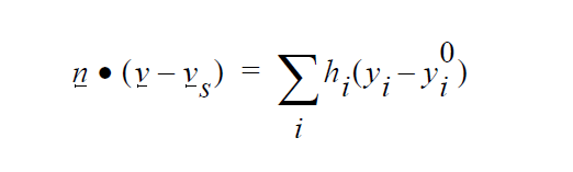
Definitions of the input parameters are as follows:
VNORM_LEAK |
Name of the boundary condition (<bc_name>). |
SS |
Type of boundary condition (<bc_type>), where SS denotes side set in the EXODUS II database. |
<bc_id> |
The boundary flag identifier, an integer associated with <bc_type> that identifies the boundary location (side set in EXODUS II) in the problem domain. |
<float1> |
\(h_i\), mass transfer coefficient for bulk fluid (n+ \(1^{th}\) species). |
<float2> |
\(y^0_i\), driving force concentration in external phase. |
Examples#
The following is a sample input card:
BC = VNORM_LEAK SS 1 1. 0.
Technical Discussion#
This card is the equivalent of KIN_LEAK except it is solved for the normal component of the momentum equation. Similar to KIN_LEAK, this flux provides an overall mass transfer balance at an interface. Please refer to the technical discussion of KIN_LEAK boundary card.
CAPILLARY#
BC = CAPILLARY SS <bc_id> <float_list> [integer]
Description / Usage#
(WIC/VECTOR MOMENTUM)
This boundary condition card is used to apply capillary forces (surface tension) to the momentum equation on a free-surface.
Definitions of the input parameters are as follows:
CAPILLARY |
Name of the boundary condition. |
SS |
Type of boundary condition (<bc_type>), where SS denotes side set in the EXODUS II database. |
<bc_id> |
The boundary flag identifier, an integer associated with <bc_type> that identifies the boundary location (side set in EXODUS II) in the problem domain. |
<float1> |
\(\sigma\), surface tension or capillary term multiplier. IMPORTANT NOTE: if no Surface Tension card appears in the material file, this parameter is the surface tension value used here. If Surface Tension is set in the material file, however, this float value will multiply the surface tension value from the material file prior to it’s application in this boundary condition. Best practice is to set this parameter to 1.0 and set the surface tension value in the material file. |
<float2> |
\(P_{ex}\), the external applied isotropic pressure on the free surface. |
<float3> |
\(P_r\), deprecated capability. Always set to zero. |
[integer] |
Optional integer value indicating the element block id from which to apply the boundary condition. This is used to force the capillary stresses to be applied from within a phase where the momentum equations are defined. |
Examples#
Following is a sample card:
BC = CAPILLARY SS 12 1.0 10.0 0.0
This card specifies that capillary forces be applied to the free surface on side set 12. If a surface tension material parameter value or model is supplied, this is the surface tension value used. If not, the surface tension value used is 1.0. An external isotropic pressure of 10.0 is applied from the surrounding environment.
Technical Discussion#
One of the primary characteristics of a free-surface is the presence of surface tension-related forces. This boundary condition permits application of such forces. The forces on the fluid at the free-surface are set via the following relation:
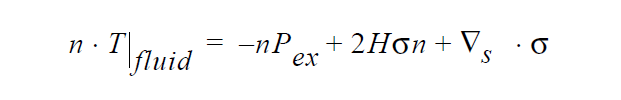
where n is the outward normal to the surface, T is the fluid stress tensor, \(P_{ex}\) is the external applied pressure described above, H is the surface curvature defined as, H = –\(\Delta_s\) ⋅ n ⁄ 2, \(\sigma\) is the surface tension, and \(\Delta_s\) is the surface divergence operator defined as \(\Delta_s^f\) = (I – nn) ⋅ \(\Delta\) f .
Typical usage of this boundary condition is in conjunction with a KINEMATIC boundary condition. The latter enforces no penetration of fluid through a free surface by deforming the mesh and this boundary condition acts on the fluid momentum equation to enforce the capillary jump condition given above.
No end of confusion results from use of this card primarily because of overloading the surface tension parameter. To reiterate, the value for surface tension that appears on this card is the actual (constant) value of surface tension that is used if a surface tension model has NOT been specified explicitly in the material file. If such a model has been identified, the surface tension parameter in the CAPILLARY card is a multiplier to the surface tension. The best practice is to simply always use 1.0 for this parameter and set the surface tension in the material file.
The optional (integer) element block ID corresponds to the material numbers given in the Problem Description section of the input file.
CAP_REPULSE#
BC = CAP_REPULSE SS <bc_id> <float_list> [mat_id]
Description / Usage#
(WIC/VECTOR MOMENTUM)
This card functions much in the same way as the CAPILLARY card. It imposes surface tension forces on free-surfaces. The addition to this card, however, is that in the vicinity of a specified planar boundary, an additional repulsive force is added to the surface tension force. This force is directed away from the planar surface and increases in proportion to 1/ \(r^2\) as the free-surface approaches the planar surface. This condition can be used to contend with the difficult problem of fluid/solid contact in an approximate way. This boundary condition is only applicable to two-dimensional problems; trying to apply it in a three-dimensional problem will cause an error.
There are seven values in the <float_list>; definitions of the input parameters are as follows:
CAP_REPULSE |
Name of the boundary condition. |
SS |
Type of boundary condition (<bc_type>), where SS denotes side set in the EXODUS II database. |
<bc_id> |
The boundary flag identifier, an integer associated with <bc_type> that identifies the boundary location (side set in EXODUS II) in the problem domain. |
<float1> |
\(\sigma\), the surface tension value or a multiplier for the capillary effect. See the important caveat under the CAPILLARY card regarding the use of this parameter when a surface tension value is supplied in the material file. |
<float2> |
\(P_{ex}\), the applied external pressure field on the free surface. |
<float3> |
\(P_{rep}\), the coefficient on the surface repulsion term. This parameter should have units of (ML/ \(T^2\)). See below for an exact description of the surface repulsion term. |
<float4> |
a, the sensitivity with respect to x-coordinate (the a coefficient) of the plane surface that is repelling the free surface sideset. |
<float5> |
b, the sensitivity with respect to y-coordinate (the b coefficient) of the plane surface that is repelling the free surface sideset. |
<float6> |
c, the sensitivity with respect to z-coordinate (the c coefficient) of the plane surface that is repelling the free surface sideset. |
<float7> |
d, the constant d coefficient of the plane surface equation that is repelling the free surface sideset. |
[mat_id] |
In the case of a surface node shared by more than one material, this optional integer parameter allows the user to specify which material the condition will be applied in. This is rarely used. |
Examples#
Following is a sample card:
BC = CAP_REPULSE SS 24 1.0 0.0 0.1 1. 1. 0. 2.
applies a standard capillary surface tension pressure jump condition to side set 24, except as the free surface approaches the plane surface defined by a solution to the equation x + y = -2.0.
Technical Discussion#
This boundary condition applies the following force term to the fluid momentum equation:
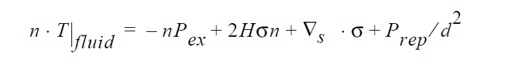
which is almost identical to the force applied by the CAPILLARY card. The only difference is the last term on the right in which d is the normal distance from a given point on the free-surface side set and the planar surface defined by the equation:
CAP_RECOIL_PRESS#
BC = CAP_RECOIL_PRESS SS <bc_id> <float_list>
Description / Usage#
(WIC/VECTOR MOMENTUM)
This boundary condition calculates the surface recoil from an evaporating metal alloy component or water.
There are seven values in the <float_list>; definitions of the input parameters are as follows:
CAP_RECOIL_PRESS |
Name of the boundary condition (<bc_name>). |
SS |
Type of boundary condition (<bc_type>), where SS denotes side set in the EXODUS II database. |
<bc_id> |
The boundary flag identifier, an integer associated with <bc_type> that identifies the boundary location (side set in EXODUS II) in the problem domain. |
<float1> |
This float is currently disabled. |
<float2> |
This float is currently disabled. |
<float3> |
Temperature at which the metal alloy begins to boil. |
<float4> |
Liquidus temperature of metal alloy. |
<float5> |
Reference temperature. |
<float6> |
Conversion scale for pressure. |
<float7> |
Conversion scale for temperature. |
Examples#
The following is a sample input card:
BC = CAP_RECOIL_PRESS SS 1 0.0 0.0 3000.0 1623.0 0.0 1.0 1.0
Technical Discussion#
Currently this boundary condition has coefficients for only iron and water. Several required pieces of information to use this boundary condition are not in final form, and the user can expect future changes and improvements. This boundary condition is designed for use with Q_LASER_WELD.
References#
No References.
ELEC_TRACTION#
BC = ELEC_TRACTION SS <bc_id> <integer> <float>
Description / Usage#
(WIC/VECTOR MOMENTUM)
This boundary condition card is used to add to the momentum equation the electric, or Maxwell, stress at a free-surface. Definitions of the input parameters are as follows:
ELEC_TRACTION |
Name of the boundary condition (<bc_name>). |
SS |
Type of boundary condition (<bc_type>), where SS denotes side set in the EXODUS II database. |
<bc_id> |
The boundary flag identifier, an integer associated with <bc_type> that identifies the boundary location (side set in EXODUS II) in the problem domain. |
<integer> |
Integer value indicating the element block ID from which to apply the boundary condition. |
<float> |
A term-multiplier. |
Since this boundary condition only adds the electric stress, it is commonly used with one of the CAPILLARY, CAP_RECOIL_PRESS or CAP_REPULSE boundary conditions, viz. the capillary stress must be added separately.
Examples#
For a system consisting of an insulating liquid (element block ID 1) and an insulating, passive gas (element block ID 2) with a free-surface designated by side set 12, the following is a sample usage:
BC = ELEC_TRACTION SS 12 1 1.0
BC = ELEC_TRACTION SS 12 2 1.0
BC = CAPILLARY SS 12 1.0 0.0 0.0 1
The first and second lines adds the electric stress due to the electric field in the liquid and gas phases, respectively. The third line adds the capillary stress due to surface tension. IMPORTANT NOTE: the optional element block ID argument to the CAPILLARY card is used to make sure that the capillary stress is added from within a phase where the momentum equations are defined. The same holds for the KINEMATIC boundary condition.
Technical Discussion#
This boundary condition adds the electric, or Maxwell, stress contribution to the traction condition. To use this boundary condition there must be a VOLTAGE equation present in one or both of the materials neighboring the interface, i.e., one or both of the neighboring materials must be a dielectric. The electrical permittivity of each dielectric material must be supplied via the Electrical Conductivity card (yes, this is a kludge) in the material property file.
In its most general form, the traction condition is written
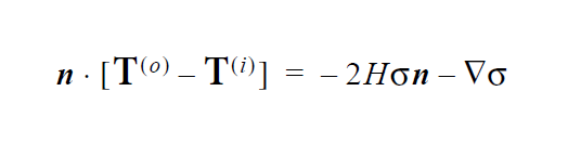
where T is the stress tensor, the superscripts ( o ) and ( i ) denote the outer and inner phases, n is a unit normal pointing into the outer phase, -H is the local mean curvature, and \(\sigma\) is the surface tension.
The stress tensor can be written as the sum of the mechanical stress \(T_m\) (e.g., the Newtonian stress tensor) and an electrical stress \(T_e\), viz. T = \(T_m\) + \(T_e\). The electric stress tensor provided through this boundary condition applies to incompressible, polarizable materials:
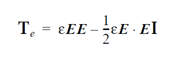
where \(\varepsilon\) is the electrical permittivity, E = – \(\Delta\) V is the electric field and V is the voltage or electric potential.
In expanded form, the traction condition becomes
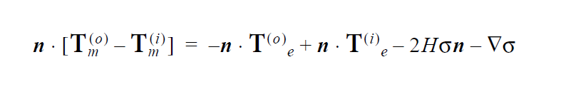
The ELEC_TRACTION boundary condition is responsible for applying either the first or second terms on the right hand side (specified through the element block ID parameter) whereas the CAPILLARY (or related boundary condition) is responsible for the third and fourth terms.
The term multiplier supplied by the <float> input is used in the elec_surf_stress() function (mm_ns_bc.c) which applies the ELEC_TRACTION boundary condition. It is the etm function argument. The normal term multipliers couldn’t be used because this boundary condition can be applied from within a material that doesn’t have the momentum equations defined (or properly set).
CAP_ENDFORCE#
BC = CAP_ENDFORCE NS <bc_id> <float_list>
Description / Usage#
(SPECIAL/VECTOR MOMENTUM)
This boundary condition card adds surface tangent forces to the momentum equations at the endpoint of a free-surface. There are four values to be input for the < float_list>; definitions of the input parameters are as follows:
CAP_ENDFORCE |
Name of the boundary condition (<bc_name>). |
NS |
Type of boundary condition (<bc_type>), where NS denotes node set in the EXODUS II database. |
<bc_id> |
The boundary flag identifier, an integer associated with <bc_type> that identifies the boundary location (node set in EXODUS II) in the problem domain. |
<float1> |
X-component of surface tangent vector at end point. |
<float2> |
Y-component of surface tangent vector at end point. |
<float3> |
Z-component of surface tangent vector at end point. |
<float4> |
Equilibrium surface tension value. (See Technical Discussion.) |
This condition need only be applied at the intersection of outflow or inflow surfaces and the free-surface. The sign on the tangent vector depends on whether the computed tangent vector is facing inward or outward. This can be figured by t = n × k.
Examples#
The following is a sample input card using several APREPRO variables:
BC = CAP_ENDFORCE NS 100 {sind(th2)} {-cosd(th2)} 0.0 {surf_tens}
Technical Discussion#
The need for this boundary condition appears out of the formulation used to apply capillary forces to surfaces. The surface divergence theorem is used to simplify the curvature term in the capillary stress jump condition. This produces integrals of the form:
where C is the bounding curve of the capillary free surface, \(\sigma\) is the surface tension, \(\phi_i\) is a finite element shape function and m is a vector that is at once normal to the capillary surface and also normal to the curve C. It always points outward from the domain in question. While this is completely general for threedimensions, a surface can be reduced to a curve for two-dimensions and the divergence theorem still applies (for this boundary condition).
This card or the CAP_ENDFORCE_SCALAR is used in conjunction with the CAPILLARY card to complete (as indicated above) the treatment of capillarity conditions. It is only required when an inflow or outflow boundary intersects a free surface.
The CAP_ENDFORCE boundary condition is applied through function fapply_ST (in file mm_ns_bc.c). The boundary term is computed as the product of the surface tension supplied on this card (<float4>) and the value supplied on the Surface Tension card in the material file. When the latter card is missing, Goma defaults its value to 1.0.
This card was previously called SURFTANG for the surface tangent component of the capillary force. Old input decks can be updated simply by changing the name of the boundary condition without changing the parameters.
SURFTANG_EDGE#
BC = SURFTANG_EDGE SS <bc_id1> <bc_id2> <float_list>
Description / Usage#
(WIC/VECTOR MOMENTUM)
This boundary condition card is used to insert surface tension forces on an edge boundary defined by the primary and secondary sidesets. The direction of application of the surface tension ( \(\sigma\) ) is specified by the vector (defined by (< \(m_x\) >, < \(m_y\) >, < \(m_z\) >)). This card is the three-dimensional analog of the CAP_ENDFORCE card. It is often used at free-surface outflow boundaries if the outflow velocity is not set by a strong condition. This condition is an unrotated, weak integrated vector condition.
There are four values to be supplied in the <float_list>; definitions of the input parameters are as follows:
SURFTANG_EDGE |
Name of the boundary condition. |
SS |
Type of boundary condition (<bc_type>), where SS denotes side set in the EXODUS II database. |
<bc_id1> |
The boundary flag identifier, an integer associated with <bc_type> that identifies the primary boundary location (side set in EXODUS II) in the problem domain. This side set is usually attached to a free surface. |
<bc_id2> |
The boundary flag identifier, an integer associated with <bc_type> that identifies the secondary boundary location (side set in EXODUS II) in the problem domain. The boundary condition is applied on the edge defined by the intersection of this side set with the primary side set. |
<float1> |
\(m_x\), the x-component of direction of application of surface tension force. |
<float2> |
\(m_y\), the y-component of direction of application of surface tension force. |
<float3> |
\(m_z\), the z-component of direction of application of surface tension force. |
<float4> |
a factor multiplying the surface tension value read from the material file when evaluating the surface integral imposed by this boundary condition. |
Examples#
The following is a sample input card:
BC = SURFTANG_EDGE SS 80 60 0. -1. 0. 1.
Technical Discussion#
The need for this boundary condition appears out of the formulation used to apply capillary forces to surfaces in three-dimensions. The surface divergence theorem is used to simplify the curvature term in the capillary stress jump condition. This produces integrals of the form:
where C is the bounding curve of the capillary free surface, \(\sigma\) is the surface tension, \(\phi_i\) is a finite element shape function and m is a vector that is at once normal to the capillary surface and also normal to the curve C. It always points outward from the domain in question.
Most often this boundary condition appears at outflow boundaries of free-surfaces. It is applied along the edge where the free-surface intercepts the outflow plane. In this case, the m vector is normal to the outflow plane. If the outflow velocity is not strongly set by a Dirichlet condition or other strongly enforced condition, this boundary condition needs to be present so that a proper inclusion of all relevant surface tension terms is performed.
The <factor> parameter is provided to allow the user to independently vary the surface tension value associated with this term alone. The value for \(\sigma\) used in the preceding expression is the surface tension value obtained from the model specified in the material file multiplied by the value of <float>. Reasons for doing this are somewhat obscure but important to the practitioners of this art.
CAP_ENDFORCE_SCALAR#
BC = CAP_ENDFORCE_SCALAR NS <bc_id> <float>
Description / Usage#
(SPECIAL/VECTOR MOMENTUM)
This boundary condition card is very similar to the CAP_ENDFORCE card. It adds surface tangent forces to the momentum equations at the endpoint of a free-surface, but does not require specification of the surface tangent vector. The current free-surface tangent vector is used as the surface tangent vector. Definitions of the input parameters are as follows:
CAP_ENDFORCE_SCALAR |
Name of the boundary condition (<bc_name>). |
NS |
Type of boundary condition (<bc_type>), where NS denotes node set in the EXODUS II database. |
<bc_id> |
The boundary flag identifier, an integer associated with <bc_type> that identifies the boundary location (node set in EXODUS II) in the problem domain. |
<float> |
Equilibrium surface tension value. (See Technical Discussion.) |
This condition need only be applied at the intersection of outflow or inflow surfaces and the free-surface.
Examples#
The following is a sample input card:
BC = CAP_ENDFORCE_SCALAR NS 100 60.0
Technical Discussion#
The need for this boundary condition appears out of the formulation used to apply capillary forces to surfaces. The surface divergence theorem is used to simplify the curvature term in the capillary stress jump condition. This produces integrals of the form:
where C is the bounding curve of the capillary free surface, \(\sigma\) is the surface tension, \(\phi_i\) is a finite element shape function and m is a vector that is at once normal to the capillary surface and also normal to the curve C. It always points outward from the domain in question. While this is completely general for threedimensions, a surface can be reduced to a curve for two-dimensions and the divergence theorem still applies (for this boundary condition).
This card or the CAP_ENDFORCE is used in conjunction with the CAPILLARY card to complete (as indicated above) the treatment of capillarity conditions. It is only required when an inflow or outflow boundary intersects a free surface.
The CAP_ENDFORCE_SCALAR boundary condition is applied through function fapply_ST_scalar (in file mm_ns_bc.c). The boundary term is computed as the product of the surface tension supplied on this card (<float>) and the value supplied on the Surface Tension card in the material file. When the latter card is missing, Goma defaults its value to 1.0.
This card was previously called SURFTANG_SCALAR for the surface tangent component of the capillary force. Old input decks can be updated simply by changing the name of the boundary condition without changing the parameters.
SURFTANG_SCALAR_EDGE#
BC = SURFTANG_SCALAR_EDGE SS <bc_id1> <bc_id2> <float>
Description / Usage#
(WIC/VECTOR MOMENTUM)
Like the SURFTANG_EDGE card, this boundary condition card is used to insert surface tension forces on an outflow edge boundary defined by the primary and secondary sidesets. In contrast to the SURFTANG_EDGE card, the direction of application of the surface tension ( \(\sigma\) ) is predetermined automatically as the binormal along the edge with respect to the outward facing normal of the primary sideset. This condition is also an unrotated, weak integrated vector condition. It should be used only in three-dimensional applications.
Definitions of the input parameters are as follows:
SURFTANG_EDGE_SCALAR |
Name of the boundary condition. |
SS |
Type of boundary condition (<bc_type>), where SS denotes side set in the EXODUS II database. Since it is an EDGE condition, it applies to a curve defined as the intersection of the primary and secondary sideset. |
<bc_id1> |
The boundary flag identifier, an integer associated with <bc_type> that identifies the primary boundary location (side set in EXODUS II) in the problem domain. This side set is used in defining the edge and the local vector basis (normal, tangent, binormal) and is usually attached to a free surface. |
<bc_id2> |
The boundary flag identifier, an integer associated with <bc_type> that identifies the secondary boundary location (side set in EXODUS II) in the problem domain. It is used in defining the edge and the local vector basis (normal, tangent, binormal).The boundary condition is applied on the edge defined by the intersection of this side set with the primary side set. |
<float> |
A factor multiplying the surface tension value read from the material file when evaluating the surface integral imposed by this boundary condition. |
Examples#
The following is a sample input card:
BC = SURFTANG_EDGE_SCALAR SS 5 10 1.0
applies the boundary integral (see the Technical Discussion) along the curve described by the intersection of side sets 5 and 10. The value for surface tension in the material file is used unmodified since the multiplying factor is 1.0.
Technical Discussion#
The need for this boundary condition appears out of the formulation used to apply capillary forces to surfaces in three-dimensions. The surface divergence theorem is used to simplify the curvature term in the capillary stress jump condition. This produces integrals of the form:
where C is the bounding curve of the capillary free surface, \(\sigma\) is the surface tension, \(\phi_i\) is a finite element shape function and m is the outward binormal vector to the curve C with respect to the normal of the primary side set.
Most often this boundary condition appears at outflow boundaries of free surfaces. It is applied along the edge where the free surface intercepts the outflow plane. If the outflow velocity is not strongly set by a Dirichlet condition or other strongly enforced condition, this boundary condition needs to be present so that a proper inclusion of all relevant surface tension terms is performed.
The <factor> parameter is provided to allow the user to independently vary the surface tension value associated with this term alone. The value for \(\sigma\) used in the preceding expression is the surface tension value obtained from the model specified in the material file multiplied by the value of <float>. Reasons for doing this are somewhat obscure but important to the practitioners of this art.
FILL_CA#
BC = FILL_CA SS <bc_id> <float>
Description / Usage#
(WIC/VECTOR MOMENTUM)
This boundary condition is used to impose a contact angle on a boundary when using Level Set Interface Tracking.
A description of the input parameters follows:
FILL_CA |
Name of the boundary condition. |
SS |
Type of boundary condition (<bc_type>), where SS denotes side set in the EXODUS II database. |
<bc_id> |
The boundary flag identifier, an integer associated with <bc_type> that identifies the boundary location (side set in EXODUS II) in the problem domain. |
<float> |
\(\theta\), the contact angle imposed, in degrees. |
Examples#
An example:
BC = FILL_CA SS 10 30.0
Technical Discussion#
This boundary condition must be used in conjunction with the VELO_SLIP_FILL boundary condition. This latter condition permits the fluid to slip in the vicinity of the contact line. The FILL_CA acts by imposing a force on the momentum equation. The size of this force is more or less in proportion between the actual contact angle on the boundary and the value specified on the card. This force is applied as a weakly integrated condition and if the VELO_SLIP_FILL condition is not present, the FILL_CA will be overwritten and ipso facto absent.
References#
No References.
MOVING_CA#
BC = MOVING_CA NS <bc_id> <float_list>
Description / Usage#
(PCC/ROTATED MOMENTUM)
The intent of this boundary condition is to apply a contact angle at wetting in a twodimensional flow that is a function of the rate of advance or recession of the contact line over the substrate. It is experimental, untested, and unsupported; use it at your own risk.
There are ten values that must be specified in the <float_list>; definitions of the input parameters are as follows:
MOVING_CA |
Name of the boundary condition. |
NS |
Type of boundary condition (<bc_type>), where NS denotes node set in the EXODUS II database. |
<bc_id> |
The boundary flag identifier, an integer associated with <bc_type> that identifies the boundary location (node set in EXODUS II) in the problem domain. A KINEMATIC free surface must terminate at this single-node node set. |
<float1> |
\(\theta_{stc}\), the static contact angle, in degrees. |
<float2> |
\(n_x\), the x-component of solid surface normal vector. |
<float3> |
\(n_y\), the y-component of solid surface normal vector. |
<float4> |
\(n_z\), the z-component of solid surface normal vector. |
<float5> |
\(\theta_{adv}\), the advancing contact angle, in degrees. |
<float6> |
\(\theta_{rec}\), the receding contact angle, in degrees. |
<float7> |
\(\alpha\), the scale-factor, see below. |
<float8> |
\(v_{wx}\), the x-component of wall velocity. |
<float9> |
\(v_{wy}\), the y-component of wall velocity. |
<float10> |
\(v_{wz}\), the z-component of wall velocity. |
Examples#
The following is a sample input card:
BC = MOVING_CA NS 100 90.0 0. 1. 0. 135.0 45.0 1.0 -1. 0. 0.
Technical Discussion#
This boundary condition applies a point collocated constraint on the angle between the solid surface vector and the free-surface normal of the form:
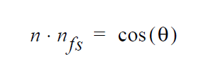
where n is the solid surface vector specified on the card and \(n_{fs}\) is the free-surface normal computed automatically by Goma. The contact angle is variable depending upon the relative velocity of the mesh speed, \(\dot{x}\) , and the substrate speed, \(v_w\) specified on the card float_list:
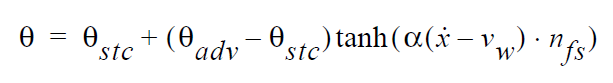
This constraint on the moving contact angle replaces a rotated component of the momentum equation. In effect a wetting force is applied at the contact line whose magnitude depends on the discrepancy between actual contact angle and that computed by the above expressions. Note that other contact angle constraints are applied to rotated components of the mesh equation. A real question exists whether such a formulation is consistent with a KINEMATIC boundary condition also applied to this node.
Not also that since this boundary condition is applied to the momentum equation, care must be taken to relax any Dirichlet on the substrate velocity. Otherwise, this latter constraint will override this constraint.
Users are again cautioned that this boundary condition is untested and potentially inconsistent. It may not work.
SDC_STEFANFLOW#
BC = SDC_STEFANFLOW SS <bc_id> <integer> {char_string}
Description / Usage#
(SIC/MOMENTUM)
This boundary condition represents the specification of the normal component of the interfacial velocity on one side of the interface. These are DVI_SIDTIE_VD boundary conditions (Moffat, 2001) that have an additional property. The first time encountered in the formation of the residual, the results of a sub calculation are stored either at the node structure level or at the surface Gauss point level. The surface reaction and surface species are specified as part of a surface domain within Chemkin.
The SURFDOMAINCHEMKIN_STEFAN_FLOW (shortened to SDC_STEFANFLOW in the name2 member of the BC_descriptions struct in mm_names.h) boundary condition solves the following equation representing Stefan flow at a boundary.
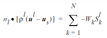
where \(n_l\) is the outward facing normal to the liquid material, \(p^l\) is the liquid density, \(u^l\) is the (mass average) velocity at the current surface quadrature point, and \(u_s\) the velocity of the mesh (i.e., the interface if the mesh is fixed at the interface). The summation over N species is for the product of molecular weight ( \(W_k\) ) and the source term for creation of species k in the liquid ( \(S_k^l\) ). Note, while it may seem that one side of the interface is getting special treatment, the combination of this boundary condition with the KINEMATIC_CHEM boundary condition actually creates a symmetric treatment of the boundary condition. SDC_STEFANFLOW is linked to the SDC_SPECIES_RXN boundary conditions just as the KINEMATIC_CHEM boundary conditions are by the expression for the interface reaction. The sum is over all of the interfacial source terms for species in the phase.
Definitions of the input parameters are as follows:
SDC_STEFANFLOW |
Name of the boundary condition (<bc_name>). |
SS |
Type of boundary condition (<bc_type>), where SS denotes side set in the EXODUS II database. |
<bc_id> |
The boundary flag identifier, an integer associated with <bc_type> that identifies the boundary location (side set in EXODUS II) in the problem domain. |
<integer> |
Element Block ID of the phase on whose side of the interface this boundary condition will be applied. |
char_string |
\(S_k^l\), string indicating where the surface source term information for this boundary condition will be obtained. Three options exist:
These are boundary conditions that apply to the Species Equations. The last boundary condition is not yet implemented, so SDC_SURFRXN currently does nothing. |
Examples#
The following is a sample input card:
BC = SDC_STEFANFLOW SS 1 0 VL_EQUIL_PSEUDORXN
The above card will create a strongly integrated boundary condition specifying the normal component of the velocity on side set 1 on the element block 0 side of the interface. The source term to be used will be taken from multiple previously specified VL_EQUIL_PSEUDORXN cards.
Technical Discussion#
Currently, this card has only been tested on internal interfaces containing discontinuous interfaces using the VL_EQUIL_PSEUDORXN source term. The SDC_SURFRXN boundary condition has not been implemented yet.
The DVI_SIDTIE_VD variable is a nomenclature adopted by Moffat (2001) in his development of a revised discontinuous variable implementation for Goma. It pertains to Discontinuous Variable Interfaces (DVI) and the strongly integrated Dirichlet (SID) boundary conditions prescribing the discontinuous value of variables on either side of an interface (TIE boundary conditions). The user is referred to Moffat (2001) for detailed presentation on discontinuous variables.
References#
GTM-015.1: Implementation Plan for Upgrading Boundary Conditions at Discontinuous-Variable Interfaces, January 8, 2001, H. K. Moffat
FLUID_SOLID#
BC = FLUID_SOLID SS <bc_id> <integer1> <integer2> [float]
Description / Usage#
(PCC/VECTOR MOMENTUM)
Used for fluid-structure interaction problems, the FLUID_SOLID condition equates the normal traction (the tangential and normal force components, per unit area) between adjacent fluid and solid materials. This condition is only to be used on boundaries between regions of ARBITRARY mesh motion with fluid momentum equations and of LAGRANGIAN or DYNAMIC_LAGRANGIAN mesh motion, with solid momentum equations (or mesh equations); see Mesh Motion and EQ cards. With this boundary condition, the local residual and Jacobian contributions from the fluid mechanics momentum equations (on the ARBITRARY side of the boundary) are added into weak form of the residual and Jacobian entries for the solid mechanics equations (on the solid LAGRANGIAN side of the boundary). All elements on both sides of the interface must have the same element type, i.e., the same order of interpolation and basis functions, e.g., Q1 or Q2. Also, such interfaces must include element sides from both sides of the interface in the defining side set.
Definitions of the input parameters are as follows:
FLUID_SOLID |
Name of the boundary condition (<bc_name>). |
SS |
Type of boundary condition (<bc_type>), where SS denotes side set in the EXODUS II database. |
<bc_id> |
The boundary flag identifier, an integer associated with <bc_type> that identifies the boundary location (side set in EXODUS II) in the problem domain. |
<integer1> |
Element block ID of solid phase (of LAGRANGIAN motion type) from the EXODUS II database. |
<integer2> |
Element block ID of liquid phase from the EXODUS II database. |
[float] |
Scale factor for stress balance for non-dimensionalization. This parameter, which multiplies the solid phase contribution, is optional; the default is 1.0. |
Examples#
The following is a sample input card:
BC = FLUID_SOLID SS 5 2 1
In this example, side set 5 is a boundary between a solid blade and a liquid; material 2 is the rubber blade, and material 1 is the fluid. Along that blade, a companion boundary condition of the form
BC = NO_SLIP SS 5 2 1
should also be applied.
Technical Discussion#
The functional form of the boundary condition is:

where \(\underline{T}\) is the fluid phase stress tensor given by any one of the specified fluid-phase constitutive equations, \(\underline{\sigma}\) and is the solid-phase stress tensor, also given by any one of the solid-phase constitutive equation (see material file specifications). \(\lambda\) is a scaling factor that defaults to unity (and is usually best taken as such unless some scaling is invoked).
This balance is applied to the weak form of the solid-phase momentum residuals, from the fluid phase, viz. in the fluid-phase, the fluid-stress at the interface is added to the solid-phase momentum residuals. As mentioned above, this condition usually needs to be supplemented by a statement of mass conservation across the interface, which will depend on whether the solid phase is of CONTINUOUS or POROUS media (see Media Type card).
FAQs#
Troubleshooting 1: This boundary condition requires that the side set contain elements from both the fluid and the solid side of the interface. For the FASTQ tool, this is the default case; for CUBIT and possibly other related tools, this can be forced on the side set definition options. Interestingly, the boundary condition does work if the side set is attached to the fluid phase only, but just due to the way in which it is applied.
Troubleshooting 2: This boundary condition does not enforce mass conservation. A combination of NO_SLIP or VELO_NORMAL/VELO_TANGENT must be invoked to achieve a material surface. For the latter, care must be taken to maintain the application of the VELO_NORMAL condition after a remesh. This condition is applied only to one side of the interface and depends on the ss_to_blks connectivity structure; it may be necessary to force its application, especially after remeshes. To be sure that the proper set of conditions is being applied, look at the BC_dup.txt file for nodes along the interface.
References#
GT-003.1: Roll coating templates and tutorial for GOMA and SEAMS, February 29, 2000, P. R. Schunk and Matt Stay
GT-006.3: Slot and Roll coating with remeshing templates and tutorial for GOMA and CUBIT/MAPVAR, August 3, 1999, R. R. Lober and P. R. Schunk
FLUID_SOLID_RS#
BC = FLUID_SOLID_RS SS <bc_id> <integer1> <integer2> [float]
Description / Usage#
(WIC/VECTOR MOMENTUM)
Please see SOLID_FLUID_RS. This boundary condition has not yet been implemented.
Examples#
No Examples.
Technical Discussion#
No Discussion.
References#
No References.
DARCY_CONTINUOUS#
BC = DARCY_CONTINOUS SS <bc_id> <integer1> <integer2> [float1]
Description / Usage#
(SIC/ROTATED MOMENTUM)
This condition enforces continuity of mass flux at an interface between a continuous medium and a saturated or partially saturated porous medium. In other words, DARCY_CONTINUOUS is a boundary condition that equates the velocity component in the liquid phase normal to the interface with the Darcy velocity in the porous phase, normal to the same interface, with proper accounting for conservation of mass using the liquid phase densities in the material files.
DARCY_CONTINOUS |
Name of the boundary condition (<bc_name>). |
SS |
Type of boundary condition (<bc_type>), where SS denotes side set in the EXODUS II database. |
<bc_id> |
The boundary flag identifier, an integer associated with <bc_type> that identifies the boundary location (side set in EXODUS II) in the problem domain. |
<integer1> |
Element block ID of porous phase from the EXODUS II database. |
<integer2> |
Element block ID of continuous fluid phase from the EXODUS II database. |
[float1] |
An optional floating point that is used for level-set free surface problems. This floating point represents a length scale over which “contact” of a liquid free surface represented by a level set field and a porous medium. It should be set to some small integer multiple of the smallest element size along the boundary. Note that this length scale is only required in cases where “sharp” interfaces using subelement integration are used. It is not required for diffuse interface representations. |
Examples#
The boundary condition
BC = DARCY_CONTINUOUS SS 5 2 1
applies to the interface defined by side set 5 which joins EXODUS II block 2 (porous phase) and block 1 (continuous phase).
Technical Discussion#
The DARCY_CONTINUOUS boundary condition imposes the following requirement at the interface between a continuous medium and a saturated or partially saturated porous medium:
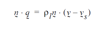
where \(\underline{n}\) is the outward-pointing normal to the surface, \(\underline{q}\) is the Darcy flux, \(p_l\) is the liquid density, presumed to be the same in the adjacent phases, \(\underline{v}\) is the fluid velocity and \(\underline{v}_s\) is the mesh velocity.
Typically this boundary condition is applied between two blocks, one being of a LAGRANGIAN mesh motion type (see Mesh Motion card) and the other being of an ARBITRARY mesh motion type. Within the LAGRANGIAN material the Media Type card is set to POROUS_SATURATED, POROUS_UNSATURATED, or POROUS_TWO_PHASE. The other block is of type CONTINOUS.
Refer to the citations below where this boundary condition is discussed in more detail.
FAQs#
Important troubleshooting note: Density, as specified in the material files for the continuous and porous phase, MUST be the same for this boundary condition to make sense.
References#
GT-008.2: Porous Media Capabilities/Tutorial for GOMA. User Guidance for Saturated Porous Penetration Problems, August 11, 1999, P. R. Schunk
GT-009.3: GOMA’s Capabilities for Partially Saturated Flow in Porous Media, September 1, 2002, P. R. Schunk
GT-028.0: Liquid Drop Impact on a Porous Substrate: a level-set tutorial, August 15, 2005.
VN_POROUS#
BC = VN_POROUS SS <bc_id> <integer_list> <float>
Description / Usage#
(SIC/ROTATED MOMENTUM)
This boundary condition is used to calculate the normal component of gas phase velocity at the interface between a continuous gas phase and porous phase. The condition is basically the unsaturated equivalent to DARCY_CONTINUOUS, and hence is a condition on the normal component of fluid (gas) velocity on the continuous side of the interface (see below). The flux on the porous medium side includes Darcy flux and Fickian diffusive flux in the porous phase. The vapor flux into gas is used to determine gas velocity. The condition is similar to the solid-liquid interface conditions that apply to interfaces between a porous medium and an external gas (in which the energy equation is used to solve for solvent concentration in the gas phase). This boundary condition is still under development and has not been recently tested. Its last use was for evaporation from a porous unsaturated film in a sol-gel application (see references below).
There are three values to be supplied for the <integer_list>; definitions of the input parameters are as follows:
VN_POROUS |
Name of the boundary condition (<bc_name>). |
SS |
Type of boundary condition (<bc_type>), where SS denotes side set in the EXODUS II database. |
<bc_id> |
The boundary flag identifier, an integer associated with <bc_type> that identifies the boundary location (side set in EXODUS II) in the problem domain. |
<integer1> |
Element block ID of solid, porous phase from the EXODUS II database. |
<integer2> |
Element block ID of gas phase from the EXODUS II database. |
<integer3> |
Set to zero for now, indicating that this condition pertains to the primary liquid solvent vapor. At some point this will be generalized to include all vapor components. |
<float> |
Density of pure solvent vapor. |
Examples#
The following is a sample input card:
BC = VN_POROUS SS 5 1 2 0 1.e-3
This condition applies to internal side set 5, which defines the interface between element block 1 (the solid porous phase which has Media Type of POROUS_PART_SAT or POROUS_TWO_PHASE) and element block 2 (the fluid phase which has Media Type CONTINUOUS). It is based on the flux of liquid solvent in the porous phase (denoted by the integer 0), the vapor form of which has a density of 1.e-3. The condition results in a blowing or sucking velocity at the interface in the fluid (gas) continuous phase.
Technical Discussion#
The functional form of this boundary condition is
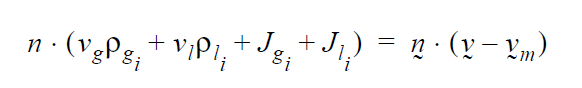
Here, the left hand side is the total flux of liquid solvent, in both gas and liquid phases. The first two terms are the Darcy pressure driven contributions, and the second two terms are the Fickian flux contributions.
This condition would be useful for predicting the gas-flow pattern above a drying porous matrix, in which the vapor flux being driven out of the porous skeleton were a mass source to drive flow in the surrounding gas. The condition has not been tested since 1995.
References#
GTM-028.0: Modeling Drying of Dip-Coated Films with Strongly-Coupled Gas Phase Natural Convection, R. A. Cairncross, 1999.
CAPILLARY_SHEAR_VISC#
BC = CAPILLARY_SHEAR_VISC SS <bc_id> <float_list> [integer]
Description / Usage#
(WIC/VECTOR MOMENTUM)
This boundary condition card is used to apply additional capillary forces beyond surface tension and surface tension gradients (as applied with use of the CAPILLARY BC) to the momentum equation on a free-surface. These additional forces are caused by surface deformation (surface expansion/contraction/shear) in the presence of surface-active species. Microstructural layers of surfactants in a capillary free surface can lead to significant dissipation of mechanical energy due to an effective surface viscosity. These additional properties are specified as inputs to this boundary condition.
Definitions of the input parameters are as follows:
CAPILLARY_SHEAR_VISC |
Name of the boundary condition. |
SS |
Type of boundary condition (<bc_type>), where SS denotes side set in the EXODUS II database. |
<bc_id> |
The boundary flag identifier, an integer associated with <bc_type> that identifies the boundary location (side set in EXODUS II) in the problem domain. |
<float1> |
\(\mu_s\), surface shear viscosity. |
<float2> |
\(\kappa_s\) , surface extensional/dilatational viscosity. |
[integer] |
Optional integer value indicating the element block id from which to apply the boundary condition. This is used to force the capillary stresses to be applied from within a phase where the momentum equations are defined. |
Examples#
Following is a sample card:
BC = CAPILLARY SS 12 1.0 10.0 0.0
BC = CAPILLARY_SHEAR_VISC SS 12 0.001 0.01
These cards specifies that capillary forces be applied to the free surface on side set 12. If a surface tension material parameter value or model is supplied, this is the surface tension value used. If not, the surface tension value used is 1.0. An external isotropic pressure of 10.0 is applied from the surrounding environment. The second card adds a surface viscosity effect. Note that you must solve the shell equation EQ = n_dot_curl_v to pick up this term.
Technical Discussion#
The functional form of this boundary condition is
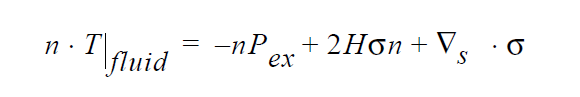
where n is the outward normal to the surface, T is the fluid stress tensor, \(\P_{ex}\) is the external applied pressure described above, H is the surface curvature defined as, H = – \(\Delta_s\) ⋅ n ⁄ 2, \(\sigma\) is the surface tension, and \(\Delta_s\) is the surface divergence operator defined as \(\Delta_s\) f = (I – nn) ⋅ \(\Delta\) f .
The Boussinesq-Scriven surface rheological constitutive equation is as follows:

Here, \(\Delta_s\) = ( \(\underline{I}\) – \(\underline{nn}\) ) ⋅ \(\Delta\) is the surface gradient operator, \(I_s\) = (\(\underline{I}\) - (\(\underline{nn}\) ) unit tensor. \(\mu_s\) and \(\kappa_s\) is the surface are the surface shear viscosity and surface dilatational viscosity, respectively. The terms beyond the first three on the right are added by this boundary condition card. Note that the first three terms on the right are balance of the stress in the standard goma CAPILLARY condition, with surface tension gradients being accommodated through variable surface tension. The boundary condition CAPILLARY_SHEAR_VISC is used to set the additional terms of this constitutive equation. As of January 2006 only the 7th term on the right hand side is implemented, as it is the only nonzero term in a flat surface shear viscometer. The building blocks for the other terms are available through additional shell equations (specifically you must solve EQ = n_dot_curl_v equation on the same shell surface). . These remaining terms actually represent additional dissipation caused by surface active species microstructures flowing in the surface. The best source of discussion of this equation is a book by Edwards et al. (1991. Interfacial Transport Processes and Rheology. Butterworth-Heinemann, Boston).
VELO_THETA_COX#
BC = VELO_THETA_COX NS <bc_id> <float_list> [integer]
Description / Usage#
(PCC/R_MOM_TANG1)
This boundary condition card applies a dynamic contact angle dependent velocity condition in a similiar fashion to VELO_THETA_TPL, but the functional form of the velocity is different. The functional form stems from the hydrodynamic theory of wetting by Cox.
The <float_list> for this boundary condition has eight values; definitions of the input parameters are as follows:
VELO_THETA_COX |
Name of the boundary condition. |
NS |
Type of boundary condition (<bc_type>), where NS denotes node set in the EXODUS II database. |
<bc_id> |
The boundary flag identifier, an integer associated with <bc_type> that identifies the boundary location (node set in EXODUS II) in the problem domain. |
<float1> |
\(\theta\), equilibrium (static) contact angle subtended by wall normal and free surface normal, in units of degrees. |
<float2> |
\(n_x\) , x-component of normal vector to the geometry boundary (see important note below regarding variable wall normals, viz. non-planar solid walls). |
<float3> |
\(n_y\) , y-component of normal vector to the geometry boundary. (see important note below regarding variable wall normals, viz. non-planar solid walls). |
<float4> |
\(n_z\) , z-component of normal vector to the geometry boundary. (see important note below regarding variable wall normals, viz. non-planar solid walls). |
<float5> |
\(\varepsilon_s\) is the dimensionless slip length, i.e. the ratio of the slip length to the characteristic length scale of the macroscopic flow. |
<float6> |
\(\sigma\) is the surface tension. This value is multiplied by the surface tension value stipulated by the surface tension material model. |
<float7> |
\(t_{relax}\) is a relaxation time which can be used to smooth the imposed contact point velocity for transient problems. Set to zero for no smoothing. |
<float8> |
\(V_{old}\) is an initial velocity used in velocity smoothing for transient problems. Set to zero when smoothing is not used. |
[integer] |
blk_id, an optional parameter that is the element block number in conjugate problems that identifies the material region to which the contact angle applies (usually the liquid element block in solid/liquid conjugate problems). |
Examples#
Following is a sample card:
BC = VELO_THETA_COX NS 100 {45} 0. 1. 0. 0.1 72.0 0 0 2
This condition applies a contact angle of 45 degrees between the free surface normal at the 100 nodeset and the vector (0,1,0). The surface tension is 72, the reciprocal of the slip coefficient is 0.1, and the dynamic contact angle is taken from element block 2. Normally, this latter vector is the normal to the solid surface in contact with the free surface at this point.
Technical Discussion#
The constraint that is imposed at the nodeset node is as follows:
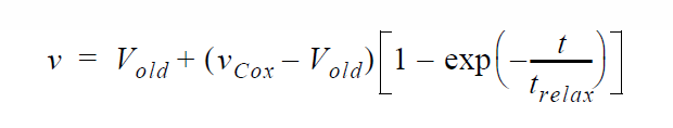
where \(v_{Cox}\) is computed from
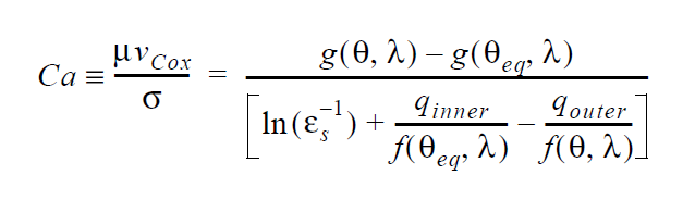
where the Cox functions, f and g, are given by;
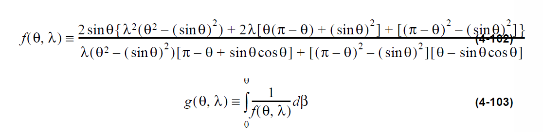
The parameters \(\lambda\), \(q_{inner}\), and \(q_{outer}\) are currently not accessible from the input card and are hard-set to zero. \(\lambda\) is the ratio of gas viscosity to liquid viscosity whereas \(q_{inner}\) and \(q_{outer}\) represent influences from the inner and outer flow regions
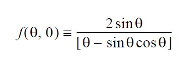
When smoothing is not used, i.e. \(t_{relax}\) = 0 , the imposed velocity is equal to that stipulated by the Hoffman correlation. Also see WETTING_SPEED_COX and SHARP_COX_VELOCITY for level-set versions.
For steady problems, the substrate velocity will be extracted from adjoining VELO_TANGENT, VELO_SLIP, or VELO_SLIP_ROT boundary conditions.
The Cox wetting velocity requires evaluation of integrals for the function g ( \(\theta\), \(\lambda\)) which is currently done numerically using 10-point Gaussian quadrature. As such the evaluation of the integrals is expected to become inaccurate as either \(\theta_eq\) tends toward zero or \(\theta\) tends toward 180 degrees. Note that the integrand becomes singular as \(\theta\) tends toward 0 or 180 degrees.
This condition was motivated by the Cox hydrodynamic theory of wetting (cf. Stephan F. Kistler, “Hydrodynamics of Wetting,” in Wettability edited by John Berg, 1993 ).
VELO_THETA_HOFFMAN#
BC = VELO_THETA_HOFFMAN NS <bc_id> <float_list> [integer]
Description / Usage#
(PCC/R_MOM_TANG1)
This boundary condition card applies a dynamic contact angle dependent velocity condition in a similiar fashion to VELO_THETA_TPL, but the functional form of the velocity is different. The functional form stems not from a theory of wetting, but instead, from a correlation of many empirical measurements.
The <float_list> for this boundary condition has eight values; definitions of the input parameters are as follows:
VELO_THETA_HOFFMAN |
Name of the boundary condition. |
NS |
Type of boundary condition (<bc_type>), where NS denotes node set in the EXODUS II database. |
<bc_id> |
The boundary flag identifier, an integer associated with <bc_type> that identifies the boundary location (node set in EXODUS II) in the problem domain. |
<float1> |
\(\theta\), equilibrium (static) contact angle subtended by wall normal and free surface normal, in units of degrees. |
<float2> |
\(n_x\) , x-component of normal vector to the geometry boundary (see important note below regarding variable wall normals, viz. non-planar solid walls). |
<float3> |
\(n_y\) , y-component of normal vector to the geometry boundary. (see important note below regarding variable wall normals, viz. non-planar solid walls). |
<float4> |
\(n_z\) , z-component of normal vector to the geometry boundary. (see important note below regarding variable wall normals, viz. non-planar solid walls). |
<float5> |
currently not used. |
<float6> |
\(\sigma\) is the surface tension. This value is multiplied by the surface tension value stipulated by the surface tension material model. |
<float7> |
\(t_{relax}\) is a relaxation time which can be used to smooth the imposed contact point velocity for transient problems. Set to zero for no smoothing. |
<float8> |
\(V_{old}\) is an initial velocity used in velocity smoothing for transient problems. Set to zero when smoothing is not used. |
[integer] |
blk_id, an optional parameter that is the element block number in conjugate problems that identifies the material region to which the contact angle applies (usually the liquid element block in solid/liquid conjugate problems). |
Examples#
Following is a sample card:
BC = VELO_THETA_HOFFMAN NS 100 {45} 0. 1. 0. 0. 72.0 0 0 2
This condition applies a contact angle of 45 degrees between the free surface normal at the 100 nodeset and the vector (0,1,0). The surface tension is 72 and the dynamic contact angle is taken from element block 2. Normally, this latter vector is the normal to the solid surface in contact with the free surface at this point.
Technical Discussion#
The constraint that is imposed at the nodeset node is as follows:
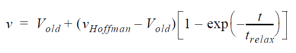
where \(v_{Hoffman}\) is computed from the implicit solution of the Hoffman correlation;
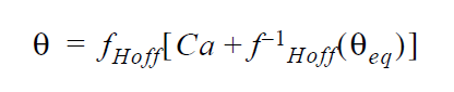
or
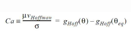
where the Hoffman functions, fHoff and gHoff, which are inverses of each other are given by;
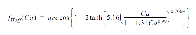
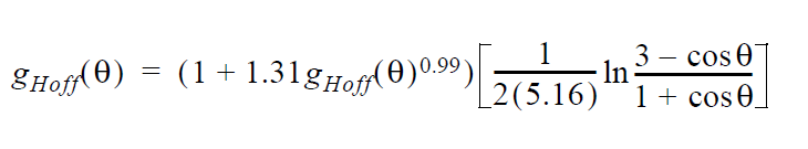
When smoothing is not used, i.e. \(t_{relax}\) = 0 , the imposed velocity is equal to that stipulated by the Hoffman correlation. Also see WETTING_SPEED_HOFFMAN and SHARP_HOFFMAN_VELOCITY for level-set versions.
For steady problems, the substrate velocity will be extracted from adjoining VELO_TANGENT, VELO_SLIP, or VELO_SLIP_ROT boundary conditions.
Because the Hoffman functions are implicit, iteration is required in the determination of the wetting velocity. As a result, for very high capillary numbers, i.e. > \(10^6\), the iteration procedure in Goma may need to be modified.
This condition was motivated by the Hoffman empirical correlation (cf. Stephan F. Kistler, “Hydrodynamics of Wetting,” in Wettability edited by John Berg, 1993).
VELO_THETA_TPL#
BC = VELO_THETA_TPL NS <bc_id> <float_list> [integer]
Description / Usage#
(PCC/R_MOM_TANG1)
This boundary condition card applies a dynamic contact angle dependent velocity condition in place of one component of the fluid momentum equation (unlike CA_BC which applies a fixed contact angle condition ot the mesh equation). The functional form of this condition is given below and stems from the Blake-DeConinck psuedomolecular kinetics theory of wetting. It is recommended that this condition or other forms of it (cf. VELO_THETA_HOFFMAN or VELO_THETA_COX) be used for steady and transient ALE problems. If you are deploying level-set technology to track moving capillary surfaces and three-phase wetting lines then the counterpart to this condition is WETTING_SPEED_LINEAR. It is noteworthy that this condition is applied to the fluid momentum equation, so that the velocity of the wetting line and the cosine of the current measured contact angle difference with the specified static value are related in a linear way.
The <float_list> for this boundary condition has eight values; definitions of the input parameters are as follows:
VELO_THETA_TPL |
Name of the boundary condition. |
NS |
Type of boundary condition (<bc_type>), where NS denotes node set in the EXODUS II database. |
<bc_id> |
The boundary flag identifier, an integer associated with <bc_type> that identifies the boundary location (node set in EXODUS II) in the problem domain. |
<float1> |
\(\theta\), equilibrium (static) contact angle subtended by wall normal and free surface normal, in units of degrees. |
<float2> |
\(n_x\) , x-component of normal vector to the geometry boundary (see important note below regarding variable wall normals, viz. non-planar solid walls). |
<float3> |
\(n_y\) , y-component of normal vector to the geometry boundary. (see important note below regarding variable wall normals, viz. non-planar solid walls). |
<float4> |
\(n_z\) , z-component of normal vector to the geometry boundary. (see important note below regarding variable wall normals, viz. non-planar solid walls). |
<float5> |
V_0 is a pre-exponential velocity factor (see functional form below) |
<float6> |
g is a thermally scaled surface tension, i.e. \(\sigma\) /2nkT. This value is multiplied by the surface tension value stipulated by the surface tension material model. |
<float7> |
\(t_{relax}\) is a relaxation time which can be used to smooth the imposed contact point velocity for transient problems. Set to zero for no smoothing. |
<float8> |
\(V_{old}\) is an initial velocity used in velocity smoothing for transient problems. Set to zero when smoothing is not used. |
[integer] |
blk_id, an optional parameter that is the element block number in conjugate problems that identifies the material region to which the contact angle applies (usually the liquid element block in solid/liquid conjugate problems). NOTE/ WARNING: As of 1/13/2013 this option seems not to work with TALE problems. |
Examples#
Following is a sample card:
BC = VELO_THETA_TPL NS 100 {45} 0. 1. 0. 1000.0 5.e-4 0 0
This condition applies a contact angle of 45 degrees between the free surface normal at the 100 nodeset and the vector (0,1,0). The velocity scale is 1000 and the sensitivity scale is 5.e-4. Normally, this latter vector is the normal to the solid surface in contact with the free surface at this point.
Technical Discussion#
The constraint that is imposed at the nodeset node is as follows:
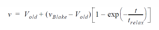
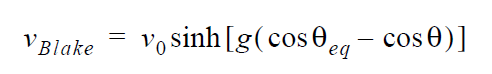
When smoothing is not used, i.e. \(t_{relax}\) = 0 , the imposed velocity is equal to that stipulated by the Blake-DeConinck equation. Also see WETTING_SPEED_LINEAR and WETTING_SPEED_BLAKE for level-set versions of this and VELO_THETA_HOFFMAN and VELO_THETA_COX for other functional forms.
We recommend use of this condition over CA_BC for all transient problems. In this case this condition displaces a momentum equation component, with the other component being used to enforce no substrate penetration. The kinematic condition is applied to the mesh motion a this node so as to conserve mass.
For steady problems, the substrate velocity will be extracted from adjoining VELO_TANGENT, VELO_SLIP, or VELO_SLIP_ROT boundary conditions.
Important: Variable Wall Normals. Situations for which the wall shape is nonplanar, meaning that the normal vector is not invariant as the contact line moves, there is an option to leave all of the normal-vector components zero. In this case Goma then seeks to determine the local wall normal vector from the geometry it is currently on, using the element facets. It is recommended that this option not be used unless the geometry is truly nonplanar, as the logic is complex and not 100% reliable. See documentation for CA_BC for an example.
This condition was motivated by T. D. Blake and is the so-called Blake- DeConinck condition (T. D. Blake, J. De Coninck 2002. “The influence of solidliquid interactions on dynamic wetting”, Advances in Colloid and Interface Science 96, 21-36. ). See this article for some options for the form of the preexponential velocity, V_0.
Important: Wall Normal convention. The wall normal vector on an external solid boundary is defined in goma as the inward facing normal to the mesh, and the free surface normal to the liquid (or wetting phase for two-liquid systems) is defined as the outward facing normal to the free surface. Put another way and referring to the picture below, the wall normal is directed from the “solid phase” to the “liquid phase”, and the free surface normal is directed from the “liquid phase” or “wetting phase” to the “vapor phase” or “Non-wetting phase”. Note that for zero contact angle the liquid is “perfectly wetting”. The air-entrainment limit (viz. the hydrodynamic theory interpretation) would occure at a 180 degree contact angle. Recall that the angle is specified in radians on this card.
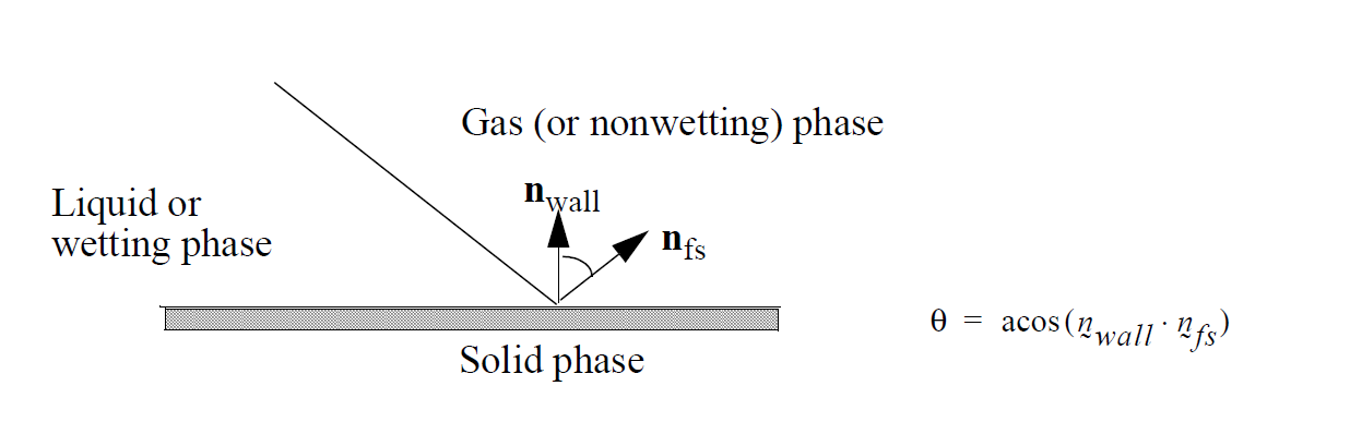
SHEET_ENDSLOPE#
BC = SHEET_ENDSLOPE NS <bc_id> <float_list>
Description / Usage#
(SPECIAL/VECTOR MOMENTUM)
This boundary condition card is used to enforce a slope of a membrane surface (cf. to be used in conjuction with BC = TENSION_SHEET) at its enpoints. . There are two values to be input for the <float_list>; definitions of the input parameters are as follows:
SHEET_ENDFORCE |
Name of the boundary condition (<bc_name>). |
NS |
Type of boundary condition (<bc_type>), where NS denotes node set in the EXODUS II database. |
<bc_id> |
The boundary flag identifier, an integer associated with <bc_type> that identifies the boundary location (node set in EXODUS II) in the problem domain. |
<float1> |
X-component of upstream idler point (see discussion below) |
<float2> |
Y-component of upstream idler point. |
Examples#
The following is a sample input card using several APREPRO variables:
BC = SHEET_ENDSLOPE NS 100 {sind(th2)} {-cosd(th2)
This condition would enforce a slope equivalent to that defined between the coordinates of the node at NS 100 with the point [sind(th2), -cosd(th2)].
Technical Discussion#
Only two dimensional applications, viz. the nodeset is a single-node nodeset.
This is a single point nodeset boundary condition. Its function is to set the slope of the web at the single point nodeset N. It does this by enforcing continuity of the slope of the TENSION_SHEET sideset with the straight line that connects the point (X,Y) with nodeset N. Thus, this boundary condition can be used to model the influence of an upstream idler roller located at the point (X,Y). Indeed, this boundary condition has an alternate name: IDLER_LOC.
This boundary condition exploits the natural boundary conditions associated with the TENSION_SHEET formulation so it really can only beused in conjunction with the latter boundary condition.
One caveat that must be mentioned is that the formulation of these two boundary conditions is not general and therefore they should only be applied to web geometries that are predominantly horizontal. That is, the x component of the normal vector to the web sideset should at each point be less than or equal to the y component.
TENSION_SHEET#
BC = TENSION_SHEET SS <bc_id> <float>
Description / Usage#
(SIC/VECTOR MOMENTUM)
This boundary condition card is used to apply a membrane force to the fluid momentum equation in order to model a membrane-like structure, viz. one with no bending stiffness but with significant tension much larger than the fluid viscous stresses. This boundary condition is basically the same mathematically as the capillary condition, with the tension here specified instead of a capillary surface tension. The only difference is the way in which it is applied: it is applied as a strong integrated condition instead of a weak form condition.
Definitions of the input parameters are as follows:
TENSION_SHEET |
Name of the boundary condition. |
SS |
Type of boundary condition (<bc_type>), where SS denotes side set in the EXODUS II database. |
<bc_id> |
The boundary flag identifier, an integer associated with <bc_type> that identifies the boundary location (side set in EXODUS II) in the problem domain. |
<float1> |
Τ, Tension of the membrane. |
Examples#
Following is a sample card:
BC = TENSION_SHEET SS 12
Technical Discussion#
Usage notes:
Can only be applied in two dimensions.
One caveat that must be mentioned is that the formulation of these two boundary conditions is not general and therefore they should only be applied to web geometries that are predominantly horizontal. That is, the x component of the normal vector to the web sideset should at each point be less than or equal to the y component.
To set the slope of the membrane at an endpoint, see the BC = SHEET_ENDSLOPE card.
This boundary condition that can be used to model the interaction of fluid with a thin sheet under a constant tension load. The sideset to which it is applied must be fully “wetted” by a fluid. Note that this boundary condition arises as a simplification of the tensioned-web shell equations (cf. shell_tension and shell_curvature equations as described in GT-033.0 and GT-027.0) subject to two simplifying assumptions:
The sheet supports no bending moments. That is, it isn’t very rigid.
The tension in the sheet is significantly larger than the viscous stresses in the fluid.
Given these assumptions this boundary condition can be used to model tensioned web applications without having to resort to the shell equations. It is a strongly integrated, rotated boundary condition on the mesh equations. It can only be used in twodimensional applications.
References#
GT-033.0 and GT-027.0.